EEE571 Extra Credit Problem: SymPy Solution for Circuit Analysis

This JupyterLab notebook provides a step-by-step symbolic solution using SymPy for the 3-phase parallel RLC circuit in the Extra Credit Problem. The circuit is a three - phase circuit and has per phase:

AC source:

10\sqrt{3}\; \left[kV\right]\; Line\;to\;Line \;RMS

(1)

\omega=377 \left[\frac{rad}{s}\right]

(2)

The source is connected with parallel comnination of R ( $1\; \Omega$ ), L ( $j1\; \Omega$ reactance), C (100 MVA total rating).

We have the following circuit conditions: Pre-switching: steady-state. For this state, we will compute the initial conditions using phasor analysis.

Post-switching (S opens at $i_{total} = 0$ ): For the state when the switch opens at the source current equal to 0A, we have free parallel RLC oscillations.

We will plot $v_C(t)$ and $i_L(t)$ to visualize each waveform.

Imports and Setup¶

import sympy as sp
import numpy as np
import matplotlib.pyplot as plt
from sympy import I, Abs, sqrt, exp, cos, sin, symbols, re, pi, arg
sp.init_printing(use_unicode=True)

Analysis Steps¶

Step 1: Derive Circuit Parameters¶

In this step, we symbolically define the given parameters and derive the per-phase capacitance $C$ , inductance $L$ , and capacitive reactance $X_C$ . The source is line-to-line RMS voltage $V_{LL,rms} = 10\sqrt{3}$ kV at $\omega = 377$ rad/s. Capacitor rating is 100 MVA (3-phase), inductor $j1 \Omega$ , resistor $R=1 \Omega$ .

Per phase: $V_{ph\_rms} = V_{LL\_rms}/\sqrt{3}$ , $Q_{C\_ph} = 100/3$ MVA, $X_C = V_{ph\_rms}^2 / Q_{C\_ph}$ , $L = 1/\omega$ , $C = 1/(\omega X_C)$ .

omega = symbols(r'\omega', real=True, positive=True)
R = symbols('R', real=True, positive=True)

XL = symbols('X_L', real=True, positive=True)
XC = symbols('X_C', real=True, positive=True)

V_llrms = symbols('V_llrms', real=True, positive=True)
Q_c3ph = symbols('Q_c3ph', real=True, positive=True)

L = XL / omega
C = 1 / (omega * XC)

RMS Phase Voltage¶

V_ph_rms = V_llrms / sp.sqrt(3)
V_ph_rms

Loading...

Per Phase Capacitor Reactive Power Capacity¶

Q_cph = Q_c3ph / 3
Q_cph

Loading...

Capacitive Reactance Equation¶

Xc_eq = (V_ph_rms)**2 / Q_cph
Xc_eq

Loading...

Inductance Equation¶

L_eq = XL / omega
L_eq

Loading...

Capacitance Equation¶

C_eq = 1 / (omega * Xc_eq)
C_eq

Loading...

Substitute Values to Calculate Capacitive Reactance¶

numerical_subs = {omega: 377, R: 1, XL: 1, V_llrms: 10e3*sp.sqrt(3), Q_c3ph: 100*10**6}
numerical_subs

Loading...

calc_Xc = Xc_eq.subs(numerical_subs).doit().evalf()
calc_Xc

Loading...

Display Results of Calculating Inductance, Capacitance and Capacitive Reactance¶

display(sp.Eq(sp.symbols('C'), C_eq))  # Symbolic expression
C_num = C_eq.subs(numerical_subs).doit().evalf()
print(f"Numerical C = {C_num:.2e} F ({C_num*1e6:.0f} μF)")
L_num = L_eq.subs(numerical_subs).doit().evalf()
print(f"Numerical L = {L_num:.2e} H")
Xc_num = Xc_eq.subs(numerical_subs).doit().evalf()
print(f"Numerical X_C = {Xc_num:.2f} Ω")

Loading...

Numerical C = 8.84e-4 F (884 μF)
Numerical L = 2.65e-3 H
Numerical X_C = 3.00 Ω

Output (Symbolic):

C = \frac{Q_{c3ph}}{V_{llrms}^{2} \omega}

(3)

Numerical Values:

C \approx 8.84 \times 10^{-4}\; \left[F\right]\; \left(884\;μF\right)

(4)

L \approx 2.65 \times 10^{-3}\;\left[H \right]

(5)

X_C = 3 \; \left[Ω\right]

(6)

V_{ph\_rms} = 10000 \left[V\right]

(7)

Step 2: Steady-State Analysis (Pre-Switching Phasors)¶

Steady-state ( $t<0$ ):

Admittances:

Y_R=1/R

(8)

Y_L=1/(j X_L)

(9)

Y_C=j/ X_C

(10)

Y_{total} = Y_R + Y_L + Y_C

(11)

I_{total\_rms} = V_{ph\_rms} \times Y_{total} \left(V_ph ∠0° initial\right)

(12)

Switch at $i_{total}=0$ :

Adjust $V_{ph}$ phase:

\theta = \frac{\pi}{2} - \angle{Y_{total}}

(13)

Therefore:

\angle{I_{total}} = \frac{\pi}{2}

(14)

i\left(t\right)=I_{peak} cos\left(\omega t + \frac{\pi}{2}\right) = -I_{peak} sin\left(\omega t\right), zero\;at\;t=0)

(15)

and:

v\left(0\right) = \sqrt{2} Re\left[V_{ph\_rms} e^{jθ}\right]

(16)

i_{L}\left(0\right) = \sqrt{2} Re\left[\frac{V_{ph\_rms} e^{jθ}}{j X_L}\right].

(17)

Inductive Impedance¶

Z_L = sp.I * XL
Z_L

Loading...

Inductive Admittance¶

Y_L = 1 / Z_L
Y_L

Loading...

Resistive Admittance¶

Y_R = 1 / R
Y_R

Loading...

Capacitive Admittance¶

Y_C = 1 / (-I * XC)
Y_C

Loading...

Total Admittance¶

Y_total = Y_R + Y_L + Y_C
Y_total

Loading...

Calculate Total RMS Load Current¶

I_total_rms = V_ph_rms * Y_total
I_total_rms

Loading...

Calculate Load Phase Angle¶

angle_Y = sp.arg(Y_total)
angle_Y

Loading...

Correct Phase Angle for Switch Closing at Source Current = 0A¶

theta = pi / 2 - angle_Y
theta

Loading...

Phase Voltage in Phasor Form¶

V_ph_adjusted = V_ph_rms * exp(I * theta)
V_ph_adjusted

Loading...

Magnitude of Phase Voltage¶

v0_sym = sqrt(2) * sp.re(V_ph_adjusted)
v0_sym

Loading...

Calculate RMS Inductor Current¶

I_L_rms = V_ph_adjusted / Z_L
I_L_rms

Loading...

i_L0_sym = sp.sqrt(2) * sp.re(I_L_rms)
i_L0_sym

Loading...

# Symbolic
display(sp.Eq(symbols(r'\angle\;Y_{total}'), angle_Y))
display(sp.Eq(symbols(r'\theta'), theta))

Loading...

# Numerical
subs_num = numerical_subs.copy()
subs_num

Loading...

# Restate Xc in ohms
Xc_num

Loading...

subs_num.update({XC: Xc_num})
subs_num

Loading...

Substitute into $V_0$ and Evaluate¶

v0_sym

Loading...

v0_num = float(v0_sym.subs(subs_num).doit().evalf())
v0_num

Loading...

i_L0_num = float(i_L0_sym.subs(subs_num).doit().evalf())
i_L0_num

Loading...

Phase Angle of Load Impedances $\angle Y$ in $\left[degrees\right]$ :¶

angle_Y_num = float(angle_Y.subs(subs_num).doit().evalf() * 180 / sp.pi)
angle_Y_num

Loading...

Phase of Voltage $\theta_V$ in $\left[degrees\right]$ :¶

theta_num = float(theta.subs(subs_num).doit().evalf() * 180 / sp.pi)
theta_num

Loading...

Total Load Current $I_{total}$ in $\left[Amps\right]$ :¶

I_total_mag = float(Abs(I_total_rms.subs(subs_num)).doit().evalf())
I_total_mag

Loading...

print(f"Numerical |I_total|_rms = {I_total_mag:.0f} A")
print(f"angle(Y_total) = {angle_Y_num:.2f} deg")
print(f"theta_V = {theta_num:.2f} deg")
print(f"v_C(0+) = {v0_num:.0f} V")
print(f"i_L(0+) = {i_L0_num:.0f} A")

Numerical |I_total|_rms = 12019 A
angle(Y_total) = -33.69 deg
theta_V = 123.69 deg
v_C(0+) = -7845 V
i_L(0+) = 11767 A

Output (Symbolic):

\angle Y_{total} = \arg\left(\frac{i Q_{c3ph}}{V_{llrms}^{2}} - \frac{i}{X_{L}} + \frac{1}{R}\right)

(18)

\theta = - \arg\left(\frac{i Q_{c3ph}}{V_{llrms}^{2}} - \frac{i}{X_{L}} + \frac{1}{R}\right) + \frac{\pi}{2}

(19)

Numerical Values:

$|I_{total}|_{rms} = 12019 \left[A\right]$
$\angle\left(Y_{total}\right) = -33.69 \left[deg\right]$
$\theta_V = 123.69 \left[deg\right]$
$v_{C}\left(0^+\right) = -7845 \left[V\right]$
$i_{L}\left(0^+\right) = 11767 \left[A\right]$

Step 3: Initial Conditions at $t=0^+$ ¶

Post-switching:

v_{C}\left(0^+\right) = v\left(0\right) \; (continuous)

(20)

i_{L}\left(0^+\right) = i_{L}\left(0\right) \; (continuous)

(21)

\frac{dv_C}{dt}\left(0^+\right) = - \frac{\left[i_{R}\left(0\right) + i_{L}\left(0\right)\right]}{C}

(22)

KCL: i_C + i_R + i_L = 0

(23)

dv0_num = (- v0_num / 1 - i_L0_num) / C_num

print(f"v_C(0+) = {v0_num:.0f} V")
print(f"i_L(0+) = {i_L0_num:.0f} A")
print(f"dv_C/dt(0+) = {dv0_num:.2e} V/s")

v_C(0+) = -7845 V
i_L(0+) = 11767 A
dv_C/dt(0+) = -4.44e+6 V/s

Output:
$v_{C}(0^+) = -7845 \left[V\right]$
$i_{L}(0^+) = 11767 \left[A\right]$
$\frac{dv_C}{dt}(0^+) = -4.44e+06 \left[\frac{V}{s}\right]$

Step 4: Time-Domain Differential Equations¶

Post-switching: Parallel RLC, voltage $v(t)$ common.

KCL:

C \frac{dv}{dt} + \frac{v}{R} + i_L = 0, \; with \frac{di_L}{dt} = \frac{v}{L}

(24)

Differentiate KCL:

C \frac{d^2v}{dt^2} + \left(\frac{1}{R}\right) \frac{dv}{dt} + \left(\frac{1}{L}\right) v = 0

(25)

Differential Equation:

\frac{d^2v}{dt^2} + \left(\frac{1}{R C}\right) \frac{dv}{dt} + \left(\frac{1}{L C}\right) v = 0

(26)

Characteristic Equation:

s^2 + \left(\frac{1}{R C}\right) s + \left(\frac{1}{L C}\right) = 0

(27)

Define:

\alpha = \frac{1}{2 R C}, \; \omega_0 = \frac{1}{\sqrt{L C}},\; \zeta = \frac{\alpha}{\omega_0} <\;1 \;(underdamped)

(28)

t = symbols('t', real=True)

L_for_de = symbols('L', real=True, positive=True)
C_for_de = symbols('C', real=True, positive=True)
v = sp.Function('v')(t)
eq_diff_v_presub = sp.Eq(sp.diff(v, t, 2) + (1/(R*C_for_de)) * sp.diff(v, t) + (1/(L_for_de*C_for_de)) * v, 0)

display(eq_diff_v_presub)

Loading...

eq_diff_v = sp.Eq(sp.diff(v, t, 2) + (1/(R*C)) * sp.diff(v, t) + (1/(L*C)) * v, 0)

display(eq_diff_v)

Loading...

Output (Symbolic):

\frac{d^{2}}{d t^{2}} v\left(t \right) + \frac{V_{llrms}^{2} \omega \frac{d}{d t} v\left(t \right)}{Q_{c3ph} R} + \frac{V_{llrms}^{2} \omega^{2} v\left(t \right)}{Q_{c3ph} X_{L}} = 0

(29)

Step 5: Laplace-Domain Solution¶

Unilateral Laplace $(t\geq 0)$ Transform DE:

s^2 V\left(s\right) - s v\left(0\right) - v^{\prime}\left(0\right) + \frac{1}{R C} \left[s V\left(s\right) - v\left(0\right)\right] + \frac{1}{L C} V \left(s\right) = 0

(30)

V\left(s\right) = \frac{\left[s v\left(0\right) + v^\prime\left(0\right)\right]}{\left[s^2 + \frac{1}{R C} s + \frac{1}{L C}\right]}

(31)

For $i_{L}\left(s\right)$ :

i_{L}\left(s\right) = \frac{\left[s I_{L}\left(0\right) + \frac{v(0)}{L}\right]}{\left[s² + \frac{1}{R C} s + \frac{1}{L C}\right]}

(32)

s = symbols('s')
I_L0 = symbols('I_{L0}')
V0 = symbols('V_0')
V_s = sp.Function('V')(s)
denom = s**2 + (1/(R*C_for_de))*s + 1/(L_for_de*C_for_de)
dv0_sym = (-V0 / R - I_L0) / C_for_de  # From Step 3 symbolic
V_s_sol_for_de = (s * V0 + dv0_sym) / denom

display(sp.Eq(V_s, V_s_sol_for_de))

Loading...

V_s = sp.Function('V')(s)
denom = s**2 + (1/(R*C))*s + 1/(L*C)
dv0_sym = (-V0 / R - I_L0) / C  # From Step 3 symbolic
V_s_sol = (s * V0 + dv0_sym) / denom

display(sp.Eq(V_s, V_s_sol))

Loading...

Output (Symbolic):

V\left(s \right) = \frac{V_{0} s + \frac{V_{llrms}^{2} \omega \left(- I_{L0} - \frac{V_{0}}{R}\right)}{Q_{c3ph}}}{s^{2} + \frac{V_{llrms}^{2} \omega s}{Q_{c3ph} R} + \frac{V_{llrms}^{2} \omega^{2}}{Q_{c3ph} X_{L}}}

(33)

Simplified:

V\left(s\right) = \frac{\left[s V_0 + v^\prime\left(0\right)\right]}{\left[s^2 + \frac{1}{R C} s + {\omega_0}^2\right]}

(34)

Step 6: Inverse Laplace Transform (Time-Domain Responses)¶

Underdamped:

v(t) = e^{-\alpha t} [A\;cos(\omega_d t) + B\;sin(\omega_d t)]

(35)

A = V_0

(36)

B = \frac{\left[v^{\prime}\left(0\right) + \alpha V_0\right]}{\omega_d}

(37)

i_L\left(t\right) = e^{-\alpha t} [D\;cos(\omega_d t) + E\;sin(\omega_d t)]

(38)

D = I_{L0}

(39)

E = \frac{\left[\frac{V_0}{L} + \alpha I_{L0}\right]}{\omega_d}

(40)

alpha = 1 / (2 * R * C)
alpha

Loading...

omega0 = 1 / sqrt(L * C)
omega0

Loading...

omegad = sqrt(omega0**2 - alpha**2)
omegad

Loading...

zeta = alpha / omega0
zeta

Loading...

A = V0
A

Loading...

B = (dv0_sym + alpha * V0) / omegad
B

Loading...

v_standard = exp(-alpha * t) * (A * cos(omegad * t) + B * sin(omegad * t))
v_standard

Loading...

D = I_L0
D

Loading...

E = (V0 / L + alpha * I_L0) / omegad
E

Loading...

i_L_standard = exp(-alpha * t) * (D * cos(omegad * t) + E * sin(omegad * t))
i_L_standard

Loading...

Show Symbolic Equations¶

display(sp.Eq(sp.Function('v')(t), v_standard))

Loading...

display(sp.Eq(sp.Function('i_L')(t), i_L_standard))

Loading...

Evaluate Numerically¶

subs_num_full = numerical_subs.copy()
subs_num_full

Loading...

subs_num_full.update({R:1, XL:1, XC:Xc_num, V0:v0_num, I_L0:i_L0_num, C:C_num, L:L_num})
subs_num_full

Loading...

alpha_num = float(alpha.subs(subs_num_full).doit().evalf())
alpha_num

Loading...

omega0_num = float(omega0.subs(subs_num_full).doit().evalf())
omega0_num

Loading...

omegad_num = float(omegad.subs(subs_num_full).doit().evalf())
omegad_num

Loading...

zeta_num = float(zeta.subs(subs_num_full).doit().evalf())
zeta_num

Loading...

A_num = v0_num
A_num

Loading...

B_num = (dv0_num + alpha_num * v0_num) / omegad_num
B_num

Loading...

D_num = i_L0_num
D_num

Loading...

E_num = (v0_num / L_num + alpha_num * i_L0_num) / omegad_num
E_num

Loading...

print(f'$5$')

$5$

print(f"alpha = {alpha_num:.1f} [rad/s]")
print(f"omega_0 = {omega0_num:.1f} [rad/s]")
print(f"zeta = {zeta_num:.3f}")
print(f"omega_d = {omegad_num:.1f} [rad/s]")
print(f"A = {A_num:.0f} [V], B = {B_num:.0f} [V]")
print(f"D = {D_num:.0f} [A], E = {E_num:.0f} [A]")

alpha = 565.5 [rad/s]
omega_0 = 653.0 [rad/s]
zeta = 0.866
omega_d = 326.5 [rad/s]
A = -7845 [V], B = -27175 [V]
D = 11767 [A], E = 11323 [A]

Output (Symbolic):

v\left(t \right) = \left(V_{0} \cos\left(t \sqrt{\frac{V_{llrms}^{2} \omega^{2}}{Q_{c3ph} X_{L}} - \frac{V_{llrms}^{4} \omega^{2}}{4 Q_{c3ph}^{2} R^{2}}}\right) + \frac{\left(\frac{V_{llrms}^{2} \omega \left(- I_{L0} - \frac{V_{0}}{R}\right)}{Q_{c3ph}} + \frac{V_{0} V_{llrms}^{2} \omega}{2 Q_{c3ph} R}\right) \sin\left(t \sqrt{\frac{V_{llrms}^{2} \omega^{2}}{Q_{c3ph} X_{L}} - \frac{V_{llrms}^{4} \omega^{2}}{4 Q_{c3ph}^{2} R^{2}}}\right)}{\sqrt{\frac{V_{llrms}^{2} \omega^{2}}{Q_{c3ph} X_{L}} - \frac{V_{llrms}^{4} \omega^{2}}{4 Q_{c3ph}^{2} R^{2}}}}\right) e^{- \frac{V_{llrms}^{2} \omega t}{2 Q_{c3ph} R}}

(41)

i_{L}\left(t \right) = \left(I_{L0} \cos\left(t \sqrt{\frac{V_{llrms}^{2} \omega^{2}}{Q_{c3ph} X_{L}} - \frac{V_{llrms}^{4} \omega^{2}}{4 Q_{c3ph}^{2} R^{2}}}\right) + \frac{\left(\frac{I_{L0} V_{llrms}^{2} \omega}{2 Q_{c3ph} R} + \frac{V_{0} \omega}{X_{L}}\right) \sin\left(t \sqrt{\frac{V_{llrms}^{2} \omega^{2}}{Q_{c3ph} X_{L}} - \frac{V_{llrms}^{4} \omega^{2}}{4 Q_{c3ph}^{2} R^{2}}}\right)}{\sqrt{\frac{V_{llrms}^{2} \omega^{2}}{Q_{c3ph} X_{L}} - \frac{V_{llrms}^{4} \omega^{2}}{4 Q_{c3ph}^{2} R^{2}}}}\right) e^{- \frac{V_{llrms}^{2} \omega t}{2 Q_{c3ph} R}}

(42)

Numerical:
$\alpha$ = $565.5\;\left[\frac{rad}{s}\right]$
$\omega_0$ = $653.0\;\left[\frac{rad}{s}\right]$
$\omega_d$ = $326.5\;\left[\frac{rad}{s}\right]$
$\zeta$ = 0.866

$A$ = -7845 $\left[V\right]$ , B = -27175 $\left[V\right]$
$D$ = 11767 $\left[A\right]$ , E = 11323 $\left[A\right]$

Step 7: Numerical Simulation and Plots¶

Lambdify for evaluation. t=0 to 0.1 s, dt=1 μs. Verify ICs via eval at t=0.

v_func = lambda tt: np.exp(-alpha_num * tt) * (A_num * np.cos(omegad_num * tt) + B_num * np.sin(omegad_num * tt))
v_func

<function __main__.<lambda>(tt)>

i_L_func = lambda tt: np.exp(-alpha_num * tt) * (D_num * np.cos(omegad_num * tt) + E_num * np.sin(omegad_num * tt))
i_L_func

<function __main__.<lambda>(tt)>

t_num = np.arange(0, 0.04, 1e-4)

v_plot = v_func(t_num)

i_L_plot = i_L_func(t_num)

Verify Results¶

print(f"v_C(0) = {v_plot[0]:.0f} V (should be {v0_num:.0f} V)")

v_C(0) = -7845 V (should be -7845 V)

print(f"i_L(0) = {i_L_plot[0]:.0f} A (should be {i_L0_num:.0f} A)")

i_L(0) = 11767 A (should be 11767 A)

dv_plot_0 = np.gradient(v_plot, t_num)[0]
print(f"dv_C/dt(0) ≈ {dv_plot_0:.2e} V/s (should be {dv0_num:.2e} V/s)")

dv_C/dt(0) ≈ -4.03e+06 V/s (should be -4.44e+6 V/s)

# Numerical Simulation and Plots

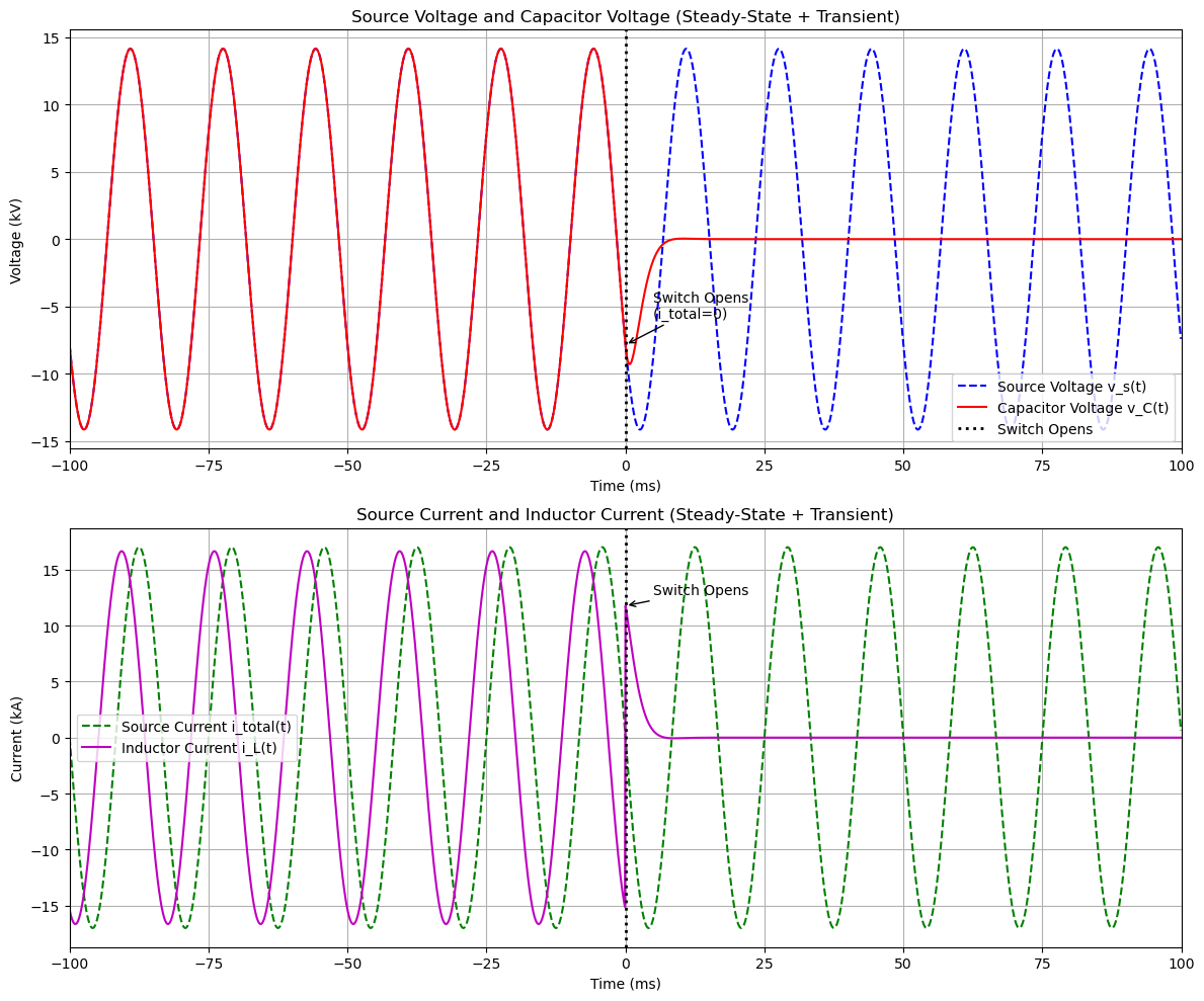
# Extended plots: Steady-state pre-switching (t < 0) and transients post-switching (t >= 0).
# Time: -0.1 to 0.1 s (few cycles before/after), dt=1 μs.
# Steady-state:
# - Source voltage v_s(t) = sqrt(2) V_ph_rms cos(ω t + θ)
# - Source current i_total(t) = sqrt(2) |I_total| cos(ω t + θ + ∠Y_total)
# - Steady-state v_C(t) = v_s(t) (parallel, directly across source)
# - Steady-state i_L(t) = sqrt(2) |I_L_rms| cos(ω t + θ + ∠I_L)
# Annotate t=0 with vertical line "Switch Opens".

# Lambdify transients (post t=0)
v_trans_func = lambda tt: np.exp(-alpha_num * tt) * (A_num * np.cos(omegad_num * tt) + B_num * np.sin(omegad_num * tt))
i_L_trans_func = lambda tt: np.exp(-alpha_num * tt) * (D_num * np.cos(omegad_num * tt) + E_num * np.sin(omegad_num * tt))

# Time vector: -0.1 to 0.1 s
t_num = np.arange(-0.1, 0.1, 1e-4)
switch_time = 0  # t=0

# Steady-state functions (for t < 0)
V_ph_peak = np.sqrt(2) * 10000
V_ph_peak

Loading...

I_total_peak = np.sqrt(2) * I_total_mag
I_total_peak

Loading...

I_L_peak = np.sqrt(2) * i_L0_num
I_L_peak

Loading...

angle_I_L = float(arg(I_L_rms.subs(subs_num)).doit().evalf() * 180 / pi)
print("Computed angle_I_L = {:.2f} deg".format(angle_I_L))

Computed angle_I_L = 33.69 deg

# Numerical omega
omega_num = 377.0

v_s_ss = lambda tt: V_ph_peak * np.cos(omega_num * tt + theta_num * np.pi / 180)
i_total_ss = lambda tt: I_total_peak * np.cos(omega_num * tt + theta_num * np.pi / 180 + angle_Y_num * np.pi / 180)
v_C_ss = v_s_ss  # Same as source
i_L_ss = lambda tt: I_L_peak * np.cos(omega_num * tt + theta_num * np.pi / 180 + angle_I_L * np.pi / 180)

# Combined waveforms
v_C_combined = np.where(t_num < switch_time, v_C_ss(t_num), v_trans_func(t_num))
i_L_combined = np.where(t_num < switch_time, i_L_ss(t_num), i_L_trans_func(t_num))

# Verify ICs (continuity at t=0)
idx_switch = np.argmin(np.abs(t_num - switch_time))
print(f"v_C(-) ≈ {v_C_ss(t_num[idx_switch-1]):.0f} V, v_C(0+) = {v_trans_func(t_num[idx_switch]):.0f} V")
print(f"i_L(-) ≈ {i_L_ss(t_num[idx_switch-1]):.0f} A, i_L(0+) = {i_L_trans_func(t_num[idx_switch]):.0f} A")
dv_plot_0 = np.gradient(v_C_combined, t_num)[idx_switch]
print(f"dv_C/dt(0) ≈ {dv_plot_0:.2e} V/s (should be {dv0_num:.2e})")

# Plots: 2 figures - one for voltages (source/v_C), one for currents (source/i_total, i_L)
fig1, (ax1a, ax1b) = plt.subplots(2, 1, figsize=(12, 10))
# Source voltage and v_C
ax1a.plot(t_num * 1000, v_s_ss(t_num) / 1000, 'b--', linewidth=1.5, label='Source Voltage v_s(t)')
ax1a.plot(t_num * 1000, v_C_combined / 1000, 'r-', linewidth=1.5, label='Capacitor Voltage v_C(t)')
ax1a.axvline(x=switch_time * 1000, color='k', linestyle=':', linewidth=2, label='Switch Opens')
ax1a.annotate('Switch Opens\n(i_total=0)', xy=(0, v0_num / 1000), xytext=(5, v0_num / 1000 + 2),
              arrowprops=dict(arrowstyle='->', color='black'), fontsize=10)
ax1a.grid(True)
ax1a.set_xlabel('Time (ms)')
ax1a.set_ylabel('Voltage (kV)')
ax1a.set_title('Source Voltage and Capacitor Voltage (Steady-State + Transient)')
ax1a.set_xlim([-100, 100])
ax1a.legend()

# Source current and i_L (steady-state only for i_total, as post-switch no source current)
ax1b.plot(t_num * 1000, i_total_ss(t_num) / 1000, 'g--', linewidth=1.5, label='Source Current i_total(t)')
ax1b.plot(t_num * 1000, i_L_combined / 1000, 'm-', linewidth=1.5, label='Inductor Current i_L(t)')
ax1b.axvline(x=switch_time * 1000, color='k', linestyle=':', linewidth=2)
ax1b.annotate('Switch Opens', xy=(0, i_L0_num / 1000), xytext=(5, i_L0_num / 1000 + 1),
              arrowprops=dict(arrowstyle='->', color='black'), fontsize=10)
ax1b.grid(True)
ax1b.set_xlabel('Time (ms)')
ax1b.set_ylabel('Current (kA)')
ax1b.set_title('Source Current and Inductor Current (Steady-State + Transient)')
ax1b.set_xlim([-100, 100])
ax1b.legend()

plt.tight_layout()
plt.show()

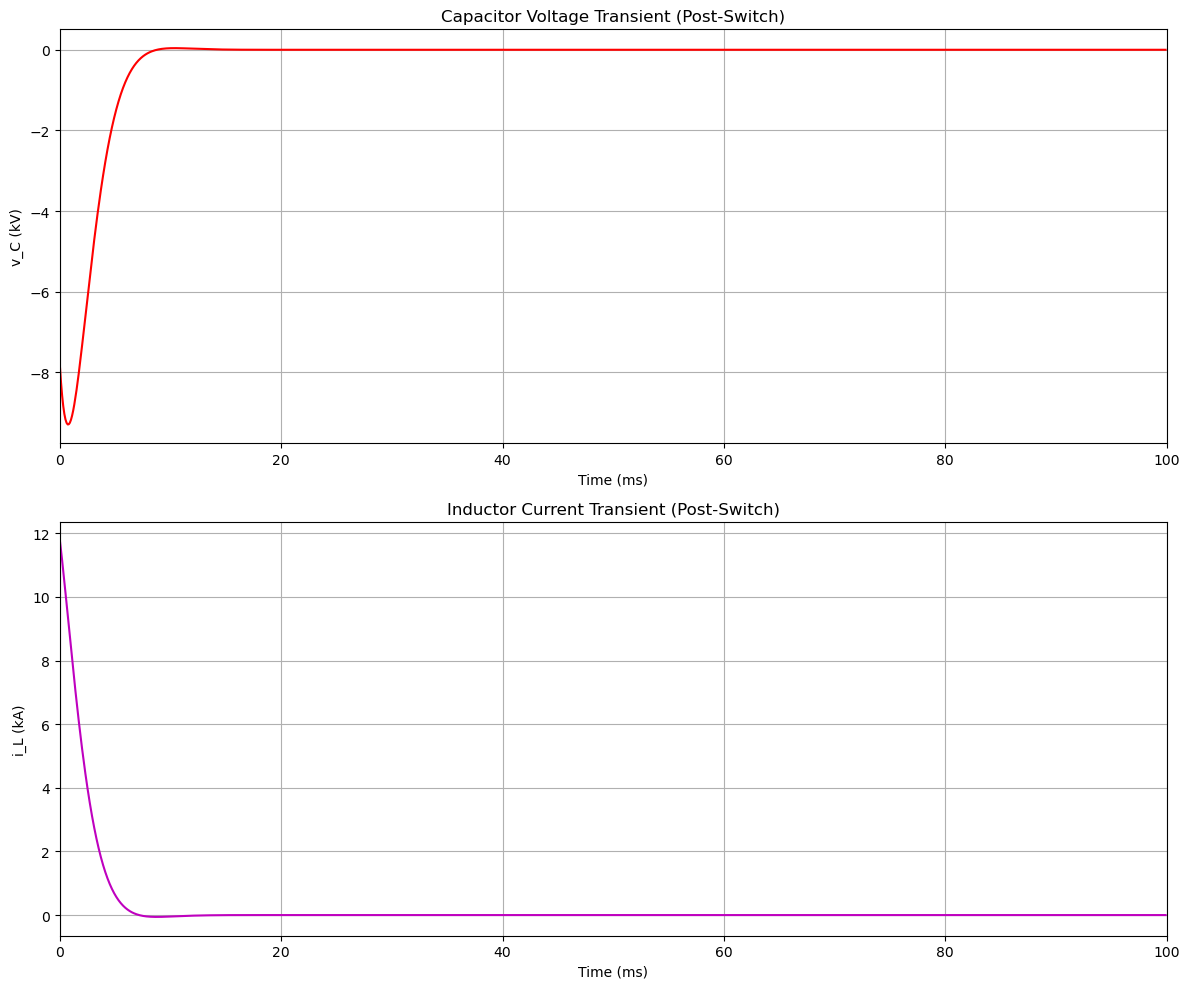
# Additional plot: Zoom on transients post-switch (t=0 to 0.1 s)
fig2, (ax2a, ax2b) = plt.subplots(2, 1, figsize=(12, 10))
ax2a.plot(t_num[t_num >= 0] * 1000, v_C_combined[t_num >= 0] / 1000, 'r-', linewidth=1.5)
ax2a.grid(True)
ax2a.set_xlabel('Time (ms)')
ax2a.set_ylabel('v_C (kV)')
ax2a.set_title('Capacitor Voltage Transient (Post-Switch)')
ax2a.set_xlim([0, 100])

ax2b.plot(t_num[t_num >= 0] * 1000, i_L_combined[t_num >= 0] / 1000, 'm-', linewidth=1.5)
ax2b.grid(True)
ax2b.set_xlabel('Time (ms)')
ax2b.set_ylabel('i_L (kA)')
ax2b.set_title('Inductor Current Transient (Post-Switch)')
ax2b.set_xlim([0, 100])

plt.tight_layout()
plt.show()

v_C(-) ≈ -7396 V, v_C(0+) = -7845 V
i_L(-) ≈ -15109 A, i_L(0+) = 11767 A
dv_C/dt(0) ≈ -4.26e+06 V/s (should be -4.44e+6)

Compare to Simulation¶

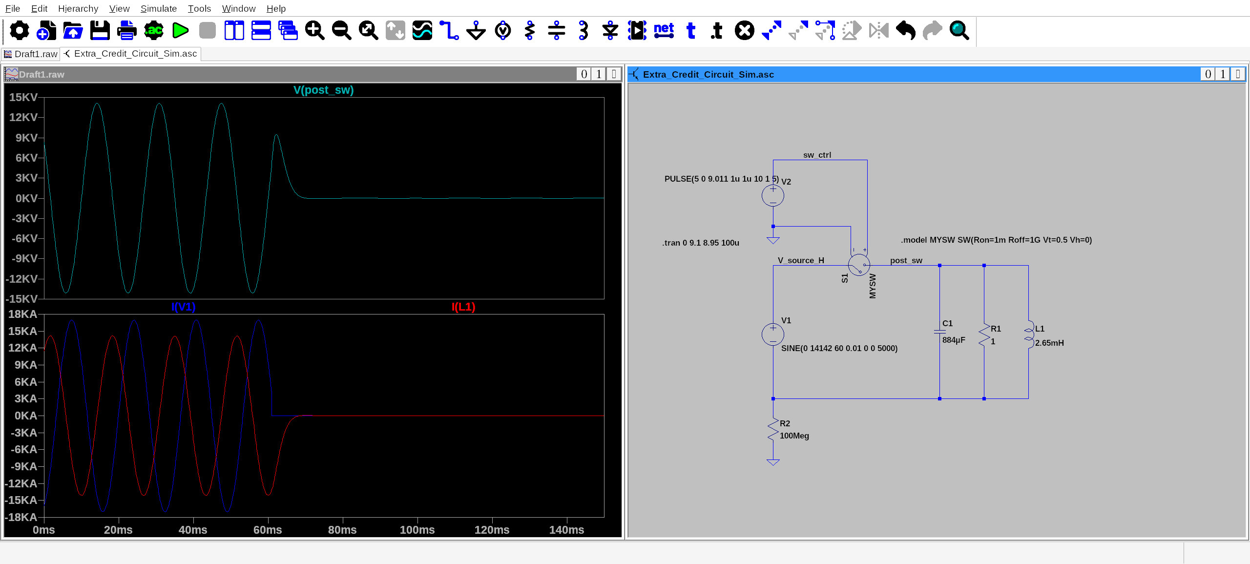
Figure 1:EEE571 Extra Credit Problem Circuit Simulation

EEE571 Extra Credit Problem: SymPy Solution for Circuit Analysis

Imports and Setup¶

Analysis Steps¶

Step 1: Derive Circuit Parameters¶

RMS Phase Voltage¶

Per Phase Capacitor Reactive Power Capacity¶

Capacitive Reactance Equation¶

Inductance Equation¶

Capacitance Equation¶

Substitute Values to Calculate Capacitive Reactance¶

Display Results of Calculating Inductance, Capacitance and Capacitive Reactance¶

Step 2: Steady-State Analysis (Pre-Switching Phasors)¶

Inductive Impedance¶

Inductive Admittance¶

Resistive Admittance¶

Capacitive Admittance¶

Total Admittance¶

Calculate Total RMS Load Current¶

Calculate Load Phase Angle¶

Correct Phase Angle for Switch Closing at Source Current = 0A¶

Phase Voltage in Phasor Form¶

Magnitude of Phase Voltage¶

Calculate RMS Inductor Current¶

Substitute into V0V_0V0​ and Evaluate¶

Phase Angle of Load Impedances ∠Y\angle Y∠Y in [degrees]\left[degrees\right][degrees]:¶

Phase of Voltage θV\theta_VθV​ in [degrees]\left[degrees\right][degrees]:¶

Total Load Current ItotalI_{total}Itotal​ in [Amps]\left[Amps\right][Amps]:¶

Step 3: Initial Conditions at t=0+t=0^+t=0+¶

Step 4: Time-Domain Differential Equations¶

Step 5: Laplace-Domain Solution¶

Step 6: Inverse Laplace Transform (Time-Domain Responses)¶

Show Symbolic Equations¶

Evaluate Numerically¶

Step 7: Numerical Simulation and Plots¶

Verify Results¶

Compare to Simulation¶

Substitute into $V_0$ and Evaluate¶

Phase Angle of Load Impedances $\angle Y$ in $\left[degrees\right]$ :¶

Phase of Voltage $\theta_V$ in $\left[degrees\right]$ :¶

Total Load Current $I_{total}$ in $\left[Amps\right]$ :¶

Step 3: Initial Conditions at $t=0^+$ ¶