Generative AI Statement: ChatGPT and Grok were used in the preparation of this Lab Report Addendum.
Import Libraries
import sympy as sp
from sympy import Matrix, pi, sqrt, acos
import control as ct
ct.config.set_defaults('iosys', repr_format='latex')
from IPython.display import display
Define Symbols
# System variables
y, h, D, u = sp.symbols('y h D u', real=True)
Fin, g, ri, ro = sp.symbols('F_{in} g r_i r_o', positive=True, real=True)

# Equilibrium symbols
he, De, ue = sp.symbols('he De ue', real=True)
# State variables
xdot_vect = \
Matrix(
[
sp.Symbol(r'\dot{x_1}'),
sp.Symbol(r'\dot{x_2}')
]
)
xdot_vectx_vect = \
Matrix(
[
sp.Symbol(r'x_1'),
sp.Symbol(r'x_2')
]
)
x_vectDisplay State Variables
display(sp.Eq(sp.Symbol('x1'), h))
display(sp.Eq(sp.Symbol('x2'), D))
display(sp.Eq(sp.Symbol('u'), u))Define and 
# Ai = pi*ri^2
# Ao = ro^2 * [ pi - 2(acos(D) - D*sqrt(1-D^2)) ]

Ai = pi * ri**2

Ao = ro**2 * (pi - 2*(sp.acos(D) - D*sp.sqrt(1 - D**2)))

display(sp.Eq(sp.Symbol('A_i'), Ai))
display(sp.Eq(sp.Symbol('A_o'), Ao))Define Non-Linear State Equations
# hdot = Fin/Ai - (Ao/Ai)*sqrt(2*g*h)
# Ddot = -u
# y = h

f1 = Fin/Ai - (Ao/Ai)*sp.sqrt(2*g*h)
f2 = -u
y = h

display(sp.Eq(sp.Symbol(r'f_1(h,D,u)'), f1))
display(sp.Eq(sp.Symbol(r'f_2(h,D,u)'), f2))
display(sp.Eq(sp.Symbol('y'), y))Linearization
Compute Jacobian Matrices Symbolically
# A = df/dx, B = df/du, C = dg/dx, D = dg/du

x = Matrix([h, D])
f = Matrix([f1, f2])

A_sym = f.jacobian(x)
B_sym = f.jacobian(Matrix([u]))
C_sym = Matrix([y]).jacobian(x)
D_sym = Matrix([y]).jacobian(Matrix([u]))
display(sp.Symbol('A'))
display(A_sym)display(sp.Symbol('B'))
display(B_sym)display(sp.Symbol('C'))
display(C_sym)display(sp.Symbol('D'))
display(D_sym)Display Individual Derivatives used in Jacobian Calculations
df1_dh = sp.simplify(sp.diff(f1, h))
df1_dD = sp.simplify(sp.diff(f1, D))
df2_dh = sp.simplify(sp.diff(f2, h))
df2_dD = sp.simplify(sp.diff(f2, D))
df1_du = sp.simplify(sp.diff(f1, u))
df2_du = sp.simplify(sp.diff(f2, u))
dy_dh = sp.simplify(sp.diff(y, h))
dy_dD = sp.simplify(sp.diff(y, D))
dy_du = sp.simplify(sp.diff(y, u))

display(sp.Eq(sp.Symbol(r'\partial f_{1} / \partial h'), df1_dh))
display(sp.Eq(sp.Symbol(r'\partial f_{1} / \partial D'), df1_dD))
display(sp.Eq(sp.Symbol(r'\partial f_{2} / \partial h'), df2_dh))
display(sp.Eq(sp.Symbol(r'\partial f_{2} / \partial D'), df2_dD))
display(sp.Eq(sp.Symbol(r'\partial f_{1} / \partial u'), df1_du))
display(sp.Eq(sp.Symbol(r'\partial f_{2} / \partial u'), df2_du))
display(sp.Eq(sp.Symbol(r'\partial y / \partial h'), dy_dh))
display(sp.Eq(sp.Symbol(r'\partial y / \partial D'), dy_dD))
display(sp.Eq(sp.Symbol(r'\partial y / \partial u'), dy_du))Subsitute Numerical Values
# Substitute the numerical values from the lab
# Lab values:
# Fin = 0.00339
# g = 9.80665
# ri = 0.15
# ro = 0.02
# he = 1
# De = 0.5
# ue = 0

vals = {
    Fin: 0.00339,
    g: 9.80665,
    ri: 0.15,
    ro: 0.02,
    he: 1.0,
    De: 0.5,
    ue: 0.0
}
Evaluate and at Equilibrium
Ai_num = sp.N(Ai.subs(vals), n=6)
Ao_num = sp.N(Ao.subs({**vals, D: vals[De]}), n=6)

display(sp.Eq(sp.Symbol('A_i'), Ai_num))
display(sp.Eq(sp.Symbol(r'A_{o}(D_e)'), Ao_num))Verify Equilibrium Condition
f1_eq = sp.simplify(f1.subs({
    Fin: vals[Fin], g: vals[g], ri: vals[ri], ro: vals[ro],
    h: vals[he], D: vals[De]
}))
f2_eq = sp.simplify(f2.subs({u: vals[ue]}))

display(sp.Eq(sp.Symbol(r'f_1(h_e,D_e,u_e)'), sp.N(f1_eq, n=6)))
display(sp.Eq(sp.Symbol(r'f_2(h_e,D_e,u_e)'), sp.N(f2_eq, n=6)))Evaluate the Jacobians at the Equilibrium
A_num = sp.N(
    A_sym.subs(
        {
            Fin: vals[Fin], g: vals[g], ri: vals[ri], ro: vals[ro],
            h: vals[he], D: vals[De], u: vals[ue]
        }
    ), n=6
)

B_num = sp.N(
    B_sym.subs(
        {
            Fin: vals[Fin], g: vals[g], ri: vals[ri], ro: vals[ro],
            h: vals[he], D: vals[De], u: vals[ue]
        }
    ), n=6
)

C_num = sp.N(
    C_sym.subs(
        {
            h: vals[he], D: vals[De], u: vals[ue]
        }
    ), n=6
)

D_num = sp.N(
    D_sym.subs(
        {
            h: vals[he], D: vals[De], u: vals[ue]
        }
    ), n=6
)
Evaluate Numerically
print("At equilibrium = ")
A_num[0, 0]
At equilibrium =
Evaluate Numerically
print("At equilibrium = ")
A_num[0, 1]
At equilibrium =
Display System Matrices
print('A evaluated at equilibrium')
display(sp.Symbol('A='))
display(A_num)
A evaluated at equilibrium
print('B evaluated at equilibrium')
display(sp.Symbol('B='))
display(B_num)
B evaluated at equilibrium
print('C evaluated at equilibrium')
display(sp.Symbol('C='))
display(C_num)
C evaluated at equilibrium
print('D evaluated at equilibrium')
display(sp.Symbol('D='))
display(D_num)
D evaluated at equilibrium
Show Partial Derivative Numerical Values
display(
    sp.Eq(
        sp.Symbol(
            r'(\partial f_{1}/\partial h)|_e'),
            sp.N(
                df1_dh.subs(
                    {
                        Fin: vals[Fin], g: vals[g], ri: vals[ri], ro: vals[ro],
                      h: vals[he], D: vals[De]
                    }
                ), n=6
            )
    )
)display(
sp.Eq(
sp.Symbol(
r'(\partial f_{1}/\partial D)|_e'),
sp.N(
df1_dD.subs(
{
Fin: vals[Fin], g: vals[g], ri: vals[ri], ro: vals[ro],
h: vals[he], D: vals[De]
}
), n=6
)
)
) display(
sp.Eq(
sp.Symbol(
r'(\partial f_{2}/\partial h)|_e'),
sp.N(
df2_dh.subs(
{
h: vals[he], D: vals[De], u: vals[ue]
}
), n=6
)
)
)display(
sp.Eq(
sp.Symbol(
r'(\partial f_{2}/\partial D)|_e'),
sp.N(
df2_dD.subs(
{
h: vals[he], D: vals[De], u: vals[ue]
}
), n=6
)
)
)display(
sp.Eq(
sp.Symbol(
r'(\partial f_{1}/\partial u)|_e'),
sp.N(
df1_du.subs(
{
h: vals[he], D: vals[De], u: vals[ue]
}
), n=6
)
)
)display(
sp.Eq(
sp.Symbol(
r'(\partial f_{2}/\partial u)|_e'),
sp.N(
df2_du.subs(
{
h: vals[he], D: vals[De], u: vals[ue]
}
), n=6
)
)
)display(
sp.Eq(
sp.Symbol(
r'(\partial y/\partial h)|_e'),
sp.N(
dy_dh.subs(
{
h: vals[he], D: vals[De], u: vals[ue]
}
), n=6
)
)
)display(
sp.Eq(
sp.Symbol(
r'(\partial y/\partial D)|_e'),
sp.N(
dy_dD.subs(
{
h: vals[he], D: vals[De], u: vals[ue]
}
), n=6
)
)
)display(
sp.Eq(
sp.Symbol(
r'(\partial y/\partial u)|_e'),
sp.N(
dy_du.subs(
{
h: vals[he], D: vals[De], u: vals[ue]
}
), n=6
)
)
)Show Numerical Results for ABCD Matrices
print("A =")
A_num
A =
print("\nB =")
B_num
B =
print("\nC =")
C_num
C =
print("\nD =")
D_num
D =
Display Linearzied Model State Space Equations
Ax = sp.MatMul(A_num, x_vect, evaluate=False)
Bu = sp.MatMul(B_num, u, evaluate=False)

rhs = sp.MatAdd(Ax, Bu, evaluate=False)

state_eq_num = sp.Eq(xdot_vect, rhs)
display(state_eq_num)Cx = sp.MatMul(C_num, x_vect, evaluate=False)
Du = sp.MatMul(D_num, u, evaluate=False)
rhs_y = sp.MatAdd(Cx, Du, evaluate=False)
output_eq = sp.Eq(y, rhs_y, evaluate=False)
display(output_eq)Plot Non-linear Function and Show Equilibrium Point
import numpy as np
import matplotlib.pyplot as plt

# ============================================================
# Step 1: Define symbols
# ============================================================
h, D = sp.symbols('h D')

Fin = 0.00339
g = 9.80665
ri = 0.15
ro = 0.02

Ai = np.pi*ri**2

# Ao function
Ao = ro**2*(sp.pi - 2*(sp.acos(D) - D*sp.sqrt(1-D**2)))

# Nonlinear function
f1 = Fin/Ai - (Ao/Ai)*sp.sqrt(2*g*h)

# ============================================================
# Step 2: Substitute equilibrium D value
# ============================================================
f1_De = f1.subs(D,0.5)

# Convert to numeric function
f_numeric = sp.lambdify(h, f1_De, 'numpy')

# ============================================================
# Step 3: Generate data
# ============================================================
h_vals = np.linspace(0.01,4,800)
f_vals = f_numeric(h_vals)

# Equilibrium
he = 1
fe = f_numeric(he)

# Derivative for linearization slope
dfdh = sp.diff(f1_De,h)
dfdh_num = float(dfdh.subs(h,he))

# Tangent line
tangent = dfdh_num*(h_vals-he)

# ============================================================
# Step 4: Plot nonlinear function
# ============================================================
plt.figure(figsize=(8,5))

plt.plot(h_vals, f_vals, linewidth=2,
         label=r'$\dot h = f_1(h,D_e)$')

plt.plot(h_vals,tangent,
         linestyle='--',
         label='Linearization (tangent)')

plt.axhline(0, linestyle='--')

# Mark equilibrium
plt.scatter(he, fe, color='red', s=80,
            label='Equilibrium')

plt.annotate(r'Equilibrium $(h_e=1)$',
             xy=(he,fe),
             xytext=(1.2,0.01),
             arrowprops=dict(arrowstyle='->'))

# ============================================================
# Annotate slope at equilibrium
# ============================================================
# Draw a small segment to visualize slope
delta_h = 0.2
h_line = np.array([he - delta_h, he + delta_h])
tangent_line = dfdh_num * (h_line - he)

plt.plot(h_line, tangent_line, color='black', linewidth=3)

# Annotate slope value
plt.annotate(rf'Slope = {dfdh_num:.6f}',
             xy=(he, fe),
             xytext=(he - 0.5, fe - 0.02),
             arrowprops=dict(arrowstyle='->'))

plt.xlabel("Liquid Height h (m)")
plt.ylabel(r'$\dot h$')
plt.title("Nonlinear Tank Dynamics and Linearization Point")

plt.grid()
plt.legend()

plt.show()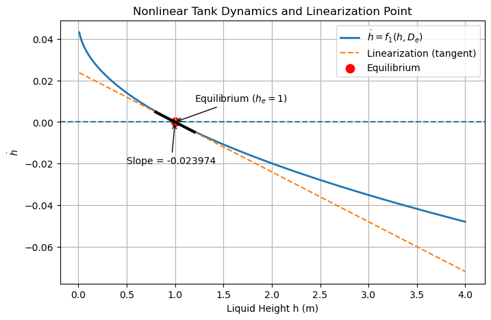
# ============================================================
# Step 1: Define symbols
# ============================================================
h, D = sp.symbols('h D', real=True)

Fin = 0.00339
g = 9.80665
ri = 0.15
ro = 0.02

Ai = np.pi * ri**2

# Outlet area Ao(D)
Ao = ro**2 * (sp.pi - 2*(sp.acos(D) - D*sp.sqrt(1 - D**2)))

# Nonlinear function h_dot = f1(h,D)
f1 = Fin/Ai - (Ao/Ai) * sp.sqrt(2*g*h)

# ============================================================
# Step 2: Fix h at the equilibrium value h_e = 1
# ============================================================
he = 1.0
De = 0.5

f1_he = sp.simplify(f1.subs(h, he))

# Convert to numeric function of D
f_numeric = sp.lambdify(D, f1_he, 'numpy')

# ============================================================
# Step 3: Compute tangent line at D_e = 0.5
# ============================================================
dfdD = sp.diff(f1_he, D)
dfdD_num = float(dfdD.subs(D, De))

# Equilibrium value
fe = float(f1_he.subs(D, De))

# Tangent line: f(D) ~ f(De) + f'(De)(D - De)
D_vals = np.linspace(0.0, 0.99, 400)
f_vals = f_numeric(D_vals)
tangent_vals = fe + dfdD_num * (D_vals - De)

# ============================================================
# Step 4: Plot nonlinear function and tangent line
# ============================================================
plt.figure(figsize=(8, 5))

plt.plot(D_vals, f_vals, linewidth=2, label=r'$\dot{h} = f_1(h_e,D)$')
plt.plot(D_vals, tangent_vals, '--', linewidth=2, label='Tangent line (linearization)')

plt.axhline(0, linestyle='--')

# Mark equilibrium point
plt.scatter(De, fe, s=80, color='red', label='Equilibrium point')

plt.annotate(r'Equilibrium $(D_e=0.5,\ \dot{h}=0)$',
             xy=(De, fe),
             xytext=(0.62, 0.01),
             arrowprops=dict(arrowstyle='->'))

# Optional slope annotation
plt.text(0.62, -0.01, rf'Slope $= \left.\frac{{\partial \dot{{h}}}}{{\partial D}}\right|_e \approx {dfdD_num:.5f}$')

plt.xlabel('D')
plt.ylabel(r'$\dot{h}$')
plt.title(r'Nonlinear $\dot{h}$ as a Function of $D$ with Tangent at Equilibrium')
plt.grid(True)
plt.legend()
plt.show()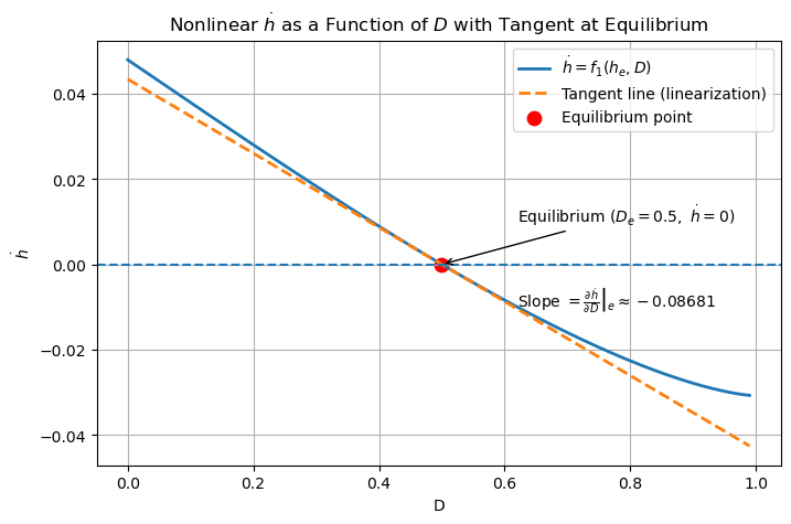
Convert into State Space Form
Define the Laplace variable 
s = sp.symbols('s', complex=True)Form 
I = sp.eye(A_num.shape[0])
Is*IA_numsI_minus_A = s*I - A_num
display(sp.Symbol(r'sI - A ='))
display(sI_minus_A)Compute 
sI_minus_A_inv = sp.simplify(sI_minus_A.inv())

display(sp.Symbol(r'(sI - A)^{-1} ='))
display(sI_minus_A_inv)Multiply 
middle_term = sp.simplify(sI_minus_A_inv * B_num)

display(sp.Symbol(r'(sI - A)^{-1} B ='))
display(middle_term)Compute 
G = sp.simplify(C_num * middle_term + D_num)

display(sp.Symbol(r'G(s) = C(sI-A)^{-1}B + D'))
display(sp.Eq(sp.Symbol(r'G(s)'), G[0]))Extract the scalar transfer function
G_scalar = sp.simplify(G[0])

display(sp.Symbol(r'G(s) = '))
display(G_scalar)Write numerator and denominator explicitly
num, den = sp.fraction(sp.together(G_scalar))
num = sp.expand(num)
den = sp.expand(den)
display(sp.Symbol('Numerator ='))
display(num)display(sp.Symbol('Denominator ='))
display(den)Factor the denominator
den_factored = sp.factor(den)

display(sp.Symbol('Factored\; denominator ='))
display(den_factored)Final result
display(sp.Eq(sp.Symbol(r'G(s)'), G_scalar))Verification using adjugate/determinant formula
# G(s) = C * adj(sI-A)/det(sI-A) * B + D
det_term = sp.expand(sI_minus_A.det())
adj_term = sI_minus_A.adjugate()
display(sp.Symbol(r'\det(sI-A) = '))
display(det_term)display(sp.Symbol(r'\operatorname{adj}(sI-A) = '))
display(adj_term)G_check = sp.simplify(C_num * adj_term * B_num / det_term + D_num)
display(sp.Symbol(r'G_{check}(s) ='))
display(G_check[0])Plot Bode and Step Response
import numpy as np
import control as ct
import matplotlib.pyplot as plt
# ============================================================
# Lab parameters
# ============================================================
Fin = 0.00339
g = 9.80665
ri = 0.15
ro = 0.02
Ai = np.pi * ri**2
# ============================================================
# Outlet area function
# ============================================================
def Ao_of_D(D):
return ro**2*(np.pi - 2*(np.arccos(D) - D*np.sqrt(1-D**2)))
# ============================================================
# Nonlinear state equations
# ============================================================
def tank_update(t,x,u,params=None):
h = x[0]
D = x[1]
uval = u[0] if np.ndim(u)>0 else u
hdot = Fin/Ai - (Ao_of_D(D)/Ai)*np.sqrt(2*g*h)
Ddot = -uval
return np.array([hdot,Ddot])
# ============================================================
# Output equation
# ============================================================
def tank_output(t,x,u,params=None):
return np.array([x[0]])
# ============================================================
# Create nonlinear system
# ============================================================
tank_nl = ct.NonlinearIOSystem(
tank_update,
tank_output,
states=2,
inputs=1,
outputs=1,
name='tank'
)
# ============================================================
# Equilibrium point
# ============================================================
xeq = np.array([1.0,0.5])
ueq = np.array([0.0])
# ============================================================
# Linearize (MATLAB linmod equivalent)
# ============================================================
tank_lin = ct.linearize(tank_nl,xeq,ueq)
A = tank_lin.A
B = tank_lin.B
C = tank_lin.C
D = tank_lin.D
print("A =\n",A)
print("\nB =\n",B)
print("\nC =\n",C)
print("\nD =\n",D)
# ============================================================
# Transfer function
# ============================================================
G = ct.tf(tank_lin)
print("\nTransfer Function:")
print(G)
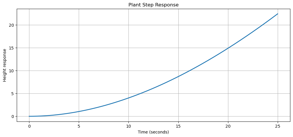
# ============================================================
# STEP RESPONSE
# ============================================================
plt.figure(figsize=(12,5))
t,y = ct.step_response(G, timepts_num=1000)
plt.plot(t,y,linewidth=2)
plt.title("Plant Step Response")
plt.xlabel("Time (seconds)")
plt.ylabel("Height response")
plt.grid()
plt.show()
# ============================================================
# BODE PLOT
# ============================================================
plt.figure(figsize=(10,5))
omega = np.logspace(-3,1,1000) # from 0.001 to 100 rad/s
ct.bode_plot(G,omega=omega, dB=True,Hz=False,deg=True,grid=True, title='Plant Bode Plot')
plt.show()A =
[[-0.02397388 -0.08681473]
[ 0. 0. ]]
B =
[[ 0.]
[-1.]]
C =
[[1. 0.]]
D =
[[0.]]
Transfer Function:
<TransferFunction>: sys[1]
Inputs (1): ['u[0]']
Outputs (1): ['y[0]']
0.08681
---------------
s^2 + 0.02397 s
Verify with Python Control Systems Library
sys = ct.ss(A_num, B_num, C_num, D_num)
sysG = ct.tf(sys)
GController Design Calculations
Design a PID controller for the linearized plant that has a bandwidth of 10 rad/sec and a phase margin of 60◦. Use = 0.0009 for the pseudo pole. The structure for a PID controller in continuous time is:
from sympy import I, Matrix, Eq, pi, atan, sqrt, NDefine symbols and known constants
w, a, K = sp.symbols('omega a K', positive=True, real=True)tau = sp.Float('0.0009')
plant_num = sp.Float('0.08681')
p1 = sp.Float('0.02397')Target Specifications for Bandwidth and Phase Margin
BW = sp.Float('10.0')          # desired bandwidth [rad/s]
PM = sp.Float('60.0')          # desired phase margin [deg]
Define Gain Crossover Frequency in 
# Use the standard PM~60° rule of thumb:
# bandwidth ~ 1.5 * gain crossover frequency
wgc = BW / sp.Float('1.5')
display(Eq(sp.Symbol(r'\omega_{gc}'), wgc))Display Design Parameters
Display Design Bandwidth in 
display(Eq(sp.Symbol(r'\omega_{BW}'), BW))Display Design Phase Margin in 
display(Eq(sp.Symbol(r'PM'), PM))Display Gain Crossover Frequency in 
display(Eq(sp.Symbol(r'\omega_{gc}'), wgc))Define Plant and Controller
# ============================================================
# P(s) = 0.08681 / [ s (s + 0.02397) ]
# C(s) = K (s+a)^2 / [ s (tau s + 1) ]
# ============================================================
s = sp.symbols('s')

P = plant_num / (s * (s + p1))
C = K * (s + a)**2 / (s * (tau*s + 1))
L = sp.simplify(P * C)
Display Plant Transfer Function 
display(Eq(sp.Symbol('P(s)'), P))Display Controller Transfer Function 
display(Eq(sp.Symbol('C(s)'), C))Display Loop Gain Transfer Function 
display(Eq(sp.Symbol('L(s)'), L))Substitute 
Ljw = sp.simplify(L.subs(s, I*wgc))

display(Eq(sp.Symbol(r'L(j\omega_{gc})'), Ljw))Write Phase Condition 
# At gain crossover:
# phase(L(jwgc)) = -180 + PM = -120 degrees
#
# Using angle addition:
# angle L = 2*atan(w/a) - 180 - atan(w/0.02397) - atan(w*tau)
# ============================================================
phase_expr_deg = (
    2*sp.atan(wgc/a) * 180/sp.pi
    - 180
    - sp.atan(wgc/p1) * 180/sp.pi
    - sp.atan(wgc*tau) * 180/sp.pi
)
display(sp.Eq(sp.Symbol(r'\angle L(j \omega)'), phase_expr_deg))phase_target = -180 + PM
phase_targetdisplay(Eq(sp.Symbol(r'\angle L(j\omega_{gc})'), phase_expr_deg))
display(Eq(sp.Symbol(r'\angle L(j\omega_{gc})'), phase_target))Solve the Phase Equation for 
phase_eq = sp.Eq(phase_expr_deg, phase_target)
phase_eqa_sol = sp.nsolve(phase_expr_deg - phase_target, 1.5) # initial guess near expected valuea_sol = sp.N(a_sol)display(Eq(sp.Symbol('a'), a_sol))Show the Phase Equation after Substituting Numbers
phase_expr_numeric = sp.simplify(phase_expr_deg.subs(a, a_sol))
phase_expr_numericdisplay(Eq(sp.Symbol(r'2\tan^{-1}(\omega_{gc}/a) -180^\circ - \tan^{-1}(\omega_{gc}/0.02397) - \tan^{-1}(\omega_{gc}\tau)'), phase_target))
display(Eq(sp.Symbol(r'a\ \text{from phase condition}'), a_sol))Write the Magnitude Condition 
# At gain crossover:
# |L(jwgc)| = 1
#
# |L(jw)| = 0.08681*K*(w^2+a^2) / [ w^2*sqrt(w^2+0.02397^2)*sqrt(1+(w*tau)^2) ]
# ============================================================
mag_expr = (
    plant_num * K * (wgc**2 + a**2)
    / (
        wgc**2
        * sp.sqrt(wgc**2 + p1**2)
        * sp.sqrt(1 + (wgc*tau)**2)
    )
)
display(Eq(sp.Symbol(r'|L(j\omega_{gc})|'), mag_expr))
display(Eq(sp.Symbol(r'|L(j\omega_{gc})|'), 1))Substitute the Computed and Solve for 
K_eq = sp.Eq(mag_expr.subs(a, a_sol), 1)
K_sol = sp.solve(K_eq, K)[0]
K_sol = sp.N(K_sol)

display(Eq(sp.Symbol('K'), K_sol))Compute from Coefficient Matching
# C(s) = K(s+a)^2 / [s(tau*s+1)]
#
# Match with:
# C(s) = kp + ki/s + kd*s/(tau*s+1)
#
# Gives:
# ki = K a^2
# kp = 2Ka - ki*tau
# kd = K - kp*tau
# ============================================================
ki = sp.simplify(K_sol * a_sol**2)
kp = sp.simplify(2*K_sol*a_sol - ki*tau)
kd = sp.simplify(K_sol - kp*tau)

ki = sp.N(ki)
kp = sp.N(kp)
kd = sp.N(kd)

display(Eq(sp.Symbol('k_i'), ki))
display(Eq(sp.Symbol('k_p'), kp))
display(Eq(sp.Symbol('k_d'), kd))Display the Computed Controller Transfer Function 
C_final = sp.simplify(C.subs({K: K_sol, a: a_sol}))
display(Eq(sp.Symbol('C(s)'), C_final))Optional - Show Key Intermediate Values Numerically
ang_pole = sp.N(sp.atan(wgc/p1) * 180/sp.pi)
ang_tau = sp.N(sp.atan(wgc*tau) * 180/sp.pi)
ang_zero = sp.N(sp.atan(wgc/a_sol) * 180/sp.pi)

display(Eq(sp.Symbol(r'\tan^{-1}(\omega_{gc}/0.02397)\ [deg]'), ang_pole))
display(Eq(sp.Symbol(r'\tan^{-1}(\omega_{gc}\tau)\ [deg]'), ang_tau))
display(Eq(sp.Symbol(r'\tan^{-1}(\omega_{gc}/a)\ [deg]'), ang_zero))Controller Design Results
print("\n================ FINAL RESULTS ================\n")
print(f"omega_gc = {float(wgc):.6f} rad/s")
print(f"a        = {float(a_sol):.6f}")
print(f"K        = {float(K_sol):.6f}")
print(f"kp       = {float(kp):.6f}")
print(f"ki       = {float(ki):.6f}")
print(f"kd       = {float(kd):.6f}")
================ FINAL RESULTS ================

omega_gc = 6.666667 rad/s
a        = 1.777740
K        = 71.699528
kp       = 254.722366
ki       = 226.596402
kd       = 71.470278
Generate Plots of Designed Controller
Declare Design Data
K = float(K_sol)
#K = 71.6833
a = float(a_sol)
#a = 1.7777
tau = 0.0009
Linearized Plant from Q2
# P(s) = 0.08681 / [ s (s + 0.02397) ]
s = ct.tf('s')
P = 0.08681 / (s * (s + 0.02397))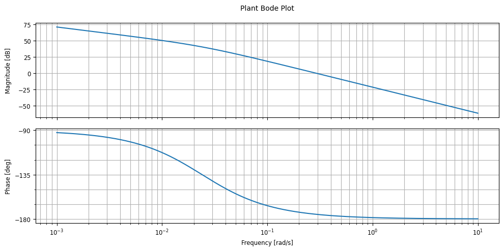
PDisplay Bode Plot of Plant 
omega = np.logspace(-3, 1, 3000)
P.bode_plot(omega=omega, title='Plant Bode Plot')
<control.ctrlplot.ControlPlot at 0x7f6d88bb2650>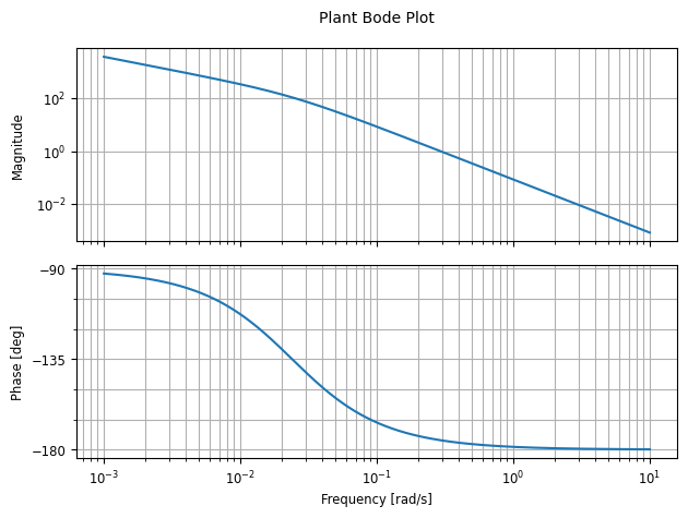
Designed Controller C(s)
# Controller:
# C(s) = K (s+a)^2 / [ s (tau s + 1) ]
C = K * (s + a)**2 / (s * (tau*s + 1))
CDisplay Bode Plot of Controller 
omega = np.logspace(-3, 5, 3000)
C.bode_plot(omega=omega, title='Controller Bode Plot')
<control.ctrlplot.ControlPlot at 0x7f6d88b96550>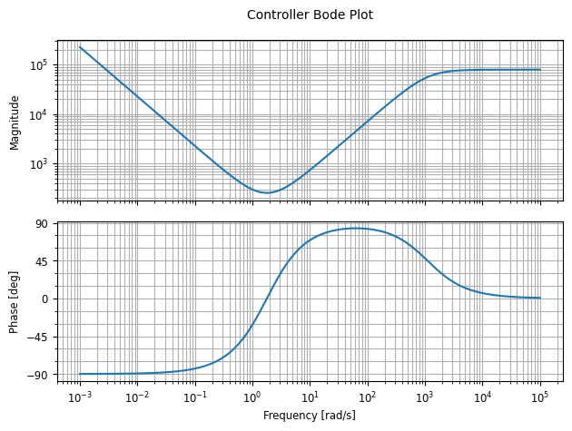
Display Loop Gain Transfer Function 
L = ct.minreal(C * P, verbose=False)
LDisplay Bode Plot of Loop Gain Transfer Function 
omega = np.logspace(-3, 5, 3000)
L.bode_plot(omega=omega, title='Loop Gain Bode Plot', wrap_phase=False)
<control.ctrlplot.ControlPlot at 0x7f6d888ae550>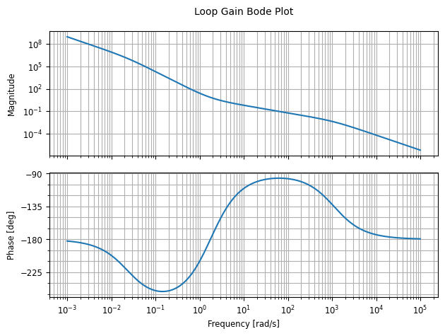
Display Complementary Sensitivity Transfer Function 
T = ct.minreal(ct.feedback(L, 1), verbose=False)   # complementary sensitivity
TDisplay Bode Plot of Complementary Sensitivty Transfer Function 
omega = np.logspace(-3, 4, 3000)
# Generate the Bode plot and get the figure/axes
T.bode_plot(omega=omega,
            title='Complementary Sensitivity Bode Plot',
            wrap_phase=True)

# Get the current figure and its axes
fig = plt.gcf()
axes = fig.axes   # This is usually a list with 2 axes: [magnitude, phase]

# axes[0] = magnitude plot (in dB)
mag_ax = axes[0]

# Add the 0 dB reference line (Gain = 1)
mag_ax.axhline(y=1,
               color='red',
               linestyle='--',
               linewidth=1.5,
               label='0 dB (Gain = 1)')

plt.tight_layout()
plt.show()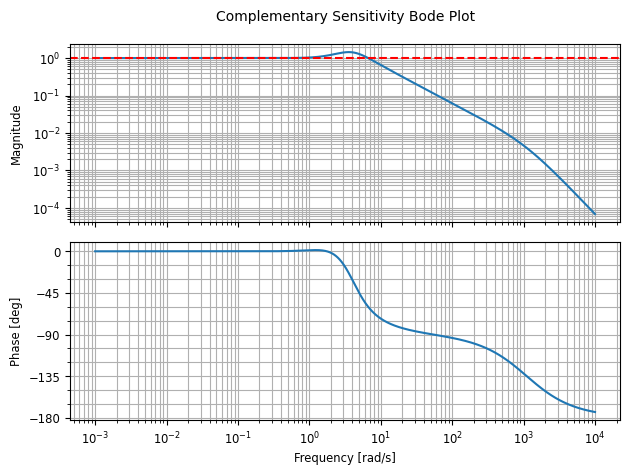
Display Sensitivity Transfer Function 
S = ct.minreal(1 / (1 + L), verbose=False)         # sensitivity
SDisplay Bode Plot of Sensitivty Transfer Function 
omega = np.logspace(-3, 4, 3000)
S.bode_plot(omega=omega, title='Sensitivity Bode Plot', wrap_phase=True)
<control.ctrlplot.ControlPlot at 0x7f6d87ff1290>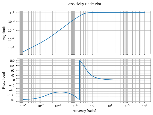
Display Gain Crossover Frequency in 
w_bw_target = 10.0
w_gc_target = w_bw_target / float(1.5)
w_gc_target6.666666666666667Calculate Verfication Quantities
# Magnitude and phase at the chosen crossover
Ljw = ct.evalfr(L, 1j * w_gc_target)
mag_at_wgc = abs(Ljw)
mag_db_at_wgc = 20 * np.log10(mag_at_wgc)
phase_deg_at_wgc = np.degrees(np.angle(Ljw))
Calculate Margins and Bandwidth
# Margins from python-control
gm, pm, wg, wp = ct.margin(L)   # wp = phase-margin crossover frequency
bw_closed = ct.bandwidth(T)
print("\n================ VERIFICATION ================\n")
print(f"Target closed-loop bandwidth = {w_bw_target:.4f} rad/s")
print(f"Chosen crossover from design rule = {w_gc_target:.4f} rad/s")
print(f"|L(jw_gc_target)| = {mag_at_wgc:.6f}")
print(f"20log10|L(jw_gc_target)| = {mag_db_at_wgc:.6f} dB")
print(f"angle L(jw_gc_target) = {phase_deg_at_wgc:.6f} deg")
print(f"Phase margin from control.margin = {pm:.6f} deg")
print(f"Phase-margin crossover frequency wp = {wp:.6f} rad/s")
print(f"Gain margin crossover frequency wg = {wg:.6f} rad/s")
print(f"Closed-loop bandwidth bandwidth(T) = {bw_closed:.6f} rad/s")
================ VERIFICATION ================

Target closed-loop bandwidth          = 10.0000 rad/s
Chosen crossover from design rule     = 6.6667 rad/s
|L(jw_gc_target)|                     = 1.000000
20log10|L(jw_gc_target)|              = -0.000000 dB
angle L(jw_gc_target)                 = -120.000000 deg
Phase margin from control.margin      = 60.000000 deg
Phase-margin crossover frequency wp   = 6.666667 rad/s
Gain margin crossover frequency wg    = 1.756420 rad/s
Closed-loop bandwidth bandwidth(T)    = 9.291460 rad/s
Build Plots
Frequency Grid
omega = np.logspace(-3, 4, 3000)Bode Plot Helper Function
def bode_data(sys, omega):
    mag, phase, omega = ct.frequency_response(sys, omega)
    mag_db = 20 * np.log10(np.squeeze(mag))
    phase_deg = np.degrees(np.unwrap(np.squeeze(phase)))
    return omega, mag_db, phase_deg
Controller Bode Plot
wc, magc_db, phasec_deg = bode_data(C, omega)

fig, ax = plt.subplots(2, 1, figsize=(10, 7), sharex=True)
fig.suptitle("Controller Bode Plot", fontsize=14)

ax[0].semilogx(wc, magc_db, linewidth=2)
ax[0].set_ylabel("Magnitude [dB]")
ax[0].grid(True, which='both')

ax[1].semilogx(wc, phasec_deg, linewidth=2)
ax[1].set_ylabel("Phase [deg]")
ax[1].set_xlabel("Frequency [rad/s]")
ax[1].grid(True, which='both')

# Annotate controller features:
# zeros at -a, integrator at 0, pseudo-pole at -1/tau
w_zero = a
w_pseudo = 1 / tau

for axes in ax:
    axes.axvline(w_zero, linestyle='--', linewidth=1)
    axes.axvline(w_pseudo, linestyle='--', linewidth=1)

ax[0].annotate(f'Zeros at ω = a = {w_zero:.4f} rad/s',
               xy=(w_zero, np.interp(w_zero, wc, magc_db)),
               xytext=(w_zero*9, np.interp(w_zero, wc, magc_db)+10),
               arrowprops=dict(arrowstyle='->'))

ax[0].annotate(rf'Pseudo-pole at ω = 1/$\tau$ = {w_pseudo:.1f} rad/s',
               xy=(w_pseudo, np.interp(w_pseudo, wc, magc_db)),
               xytext=(w_pseudo/10, np.interp(w_pseudo, wc, magc_db)-25),
               arrowprops=dict(arrowstyle='->'))

ax[1].text(1.2e-3, phasec_deg.min()+10, "Integrator at origin", fontsize=10)

plt.tight_layout()
plt.show()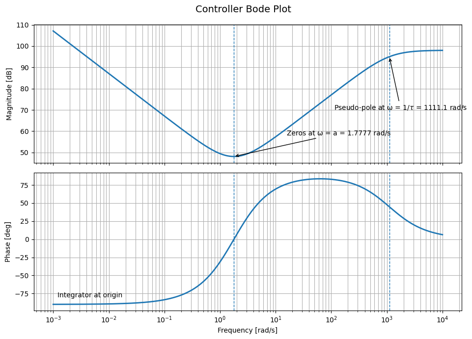
Controller Step Response
# Note: because C(s) contains an integrator, a step input causes
# the controller output to grow without bound.
# ============================================================
t_c = np.linspace(0, 0.1, 3000)
t1, y1 = ct.step_response(C, T=t_c)

plt.figure(figsize=(10, 4.5))
plt.plot(t1, y1, linewidth=2)
plt.title("Controller Step Response")
plt.xlabel("Time [s]")
plt.ylabel("Output")
plt.grid(True)

plt.annotate("Contains an integrator,\nso the step response does not settle",
             xy=(t1[len(t1)//2], y1[len(y1)//2]),
             xytext=(t1[len(t1)//2], y1[len(y1)//2] * 100),
             arrowprops=dict(arrowstyle='->'))

plt.show()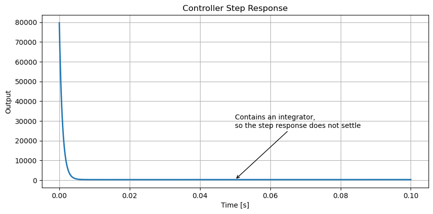
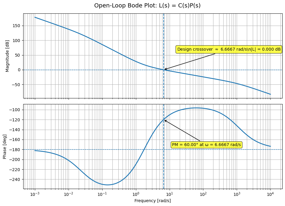
Loop Gain (Open Loop) Bode Plot of 
# Open-loop Bode plot with gain crossover and phase margin
wl, magl_db, phasel_deg = bode_data(L, omega)

fig, ax = plt.subplots(2, 1, figsize=(10, 7), sharex=True)
fig.suptitle("Open-Loop Bode Plot: L(s) = C(s)P(s)", fontsize=14)

ax[0].semilogx(wl, magl_db, linewidth=2)
ax[0].axhline(0, linestyle='--', linewidth=1)
ax[0].set_ylabel("Magnitude [dB]")
ax[0].grid(True, which='both')

ax[1].semilogx(wl, phasel_deg-360, linewidth=2)
ax[1].axhline(-180, linestyle='--', linewidth=1)
ax[1].set_ylabel("Phase [deg]")
ax[1].set_xlabel("Frequency [rad/s]")
ax[1].grid(True, which='both')

# Annotate design crossover and actual PM crossover
for axes in ax:
    axes.axvline(w_gc_target, linestyle=':', linewidth=1.5)
    if np.isfinite(wp) and wp > 0:
        axes.axvline(wp, linestyle='--', linewidth=1.5)

ax[0].annotate(rf'Design crossover $\approx$ {w_gc_target:.4f} rad/s\n|L| = {np.abs(mag_db_at_wgc):.3f} dB',
               xy=(w_gc_target, np.interp(w_gc_target, wl, magl_db)),
               xytext=(w_gc_target*2.5, np.interp(w_gc_target, wl, magl_db)+60),
               arrowprops=dict(arrowstyle='->', color='black', lw=1.2),
               ha='left', va='bottom', fontsize=10, bbox=dict(boxstyle="round,pad=0.3", fc="yellow", alpha=0.7))

# === FIXED Phase Margin Annotation ===
if np.isfinite(wp) and wp > 0:
    # Use the ACTUAL plotted y-value (after -360 shift)
    plotted_phase_at_wp = np.interp(wp, wl, phasel_deg) - 360

    print(f"Plotted phase at wp: {plotted_phase_at_wp:.2f} deg")   # for debugging

    ax[1].annotate(f'PM = {pm:.2f}° at ω = {wp:.4f} rad/s',
                   xy=(wp, plotted_phase_at_wp),           # point on the curve
                   xytext=(wp * 1.8, plotted_phase_at_wp - 55),   # text position: right and slightly above
                   arrowprops=dict(arrowstyle='->', color='black', lw=1.2),
                   ha='left', va='bottom', fontsize=10, bbox=dict(boxstyle="round,pad=0.3", fc="yellow", alpha=0.7))

plt.tight_layout()
plt.show()
Plotted phase at wp: -120.00 deg
Plot the Open Loop Step Response of 
# Note: open-loop step response is not a closed-loop performance metric.
# Because the loop contains integrators, this response will not settle.
# ============================================================
t_l = np.linspace(0, 5, 3000)
t2, y2 = ct.step_response(L, T=t_l)

plt.figure(figsize=(10, 4.5))
plt.plot(t2, y2, linewidth=2)
plt.title("Open-Loop Step Response of L(s)")
plt.xlabel("Time [s]")
plt.ylabel("Output")
plt.grid(True)

plt.annotate("Open-loop step response is shown for inspection only;\nit is not the closed-loop tracking response.",
             xy=(t2[len(t2)//3], y2[len(y2)//3]),
             xytext=(t2[len(t2)//3] + 0.5, y2[len(y2)//3] * 0.7),
             arrowprops=dict(arrowstyle='->'))

plt.show()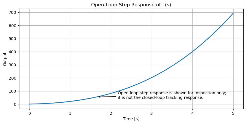
Complementary Sensitivity Bode Plot
# ============================================================
# Closed-loop Bode plot to verify bandwidth
# T(s) = L/(1+L)
# ============================================================
wt, magt_db, phaset_deg = bode_data(T, omega)

fig, ax = plt.subplots(2, 1, figsize=(10, 7), sharex=True)
fig.suptitle("Closed-Loop Complementary Sensitivity Bode Plot: T(s) = L(s)/(1+L(s))", fontsize=14)

ax[0].semilogx(wt, magt_db, linewidth=2)
ax[0].axhline(-3, linestyle='--', linewidth=1)
ax[0].set_ylabel("Magnitude [dB]")
ax[0].grid(True, which='both')

ax[1].semilogx(wt, phaset_deg, linewidth=2)
ax[1].set_ylabel("Phase [deg]")
ax[1].set_xlabel("Frequency [rad/s]")
ax[1].grid(True, which='both')

if np.isfinite(bw_closed) and bw_closed > 0:
    for axes in ax:
        axes.axvline(bw_closed, linestyle='--', linewidth=1.5)

    ax[0].annotate(f'Closed-loop bandwidth ≈ {bw_closed:.4f} rad/s',
                   xy=(bw_closed, np.interp(bw_closed, wt, magt_db)),
                   xytext=(bw_closed/1000, np.interp(bw_closed, wt, magt_db)-40),
                   arrowprops=dict(arrowstyle='->', color='black', lw=1.2),
                   ha='left', va='bottom', fontsize=10, bbox=dict(boxstyle="round,pad=0.3", fc="yellow", alpha=0.7))

# ====================== Phase Annotation ======================
if np.isfinite(pm) and pm > 0 and np.isfinite(wp) and wp > 0:
    # Find the phase value on the plotted curve at ω = wp (phase crossover)
    phase_at_wp = np.interp(wp, wt, phaset_deg)

    ax[1].annotate(f'Phase = {pm:.2f}°\nat ω = {wp:.4f} rad/s',
                   xy=(wp, phase_at_wp),                    # point on the curve
                   xytext=(wp * 2.0, phase_at_wp + 25),     # text position: right and above
                   arrowprops=dict(arrowstyle='->', color='black', lw=1.2),
                   ha='left', va='bottom', fontsize=10, bbox=dict(boxstyle="round,pad=0.3", fc="yellow", alpha=0.7))

    # Optional: add vertical line at phase crossover frequency
    for axes in ax:
        axes.axvline(wp, linestyle=':', linewidth=1.2, color='red', alpha=0.8)

plt.tight_layout()
plt.show()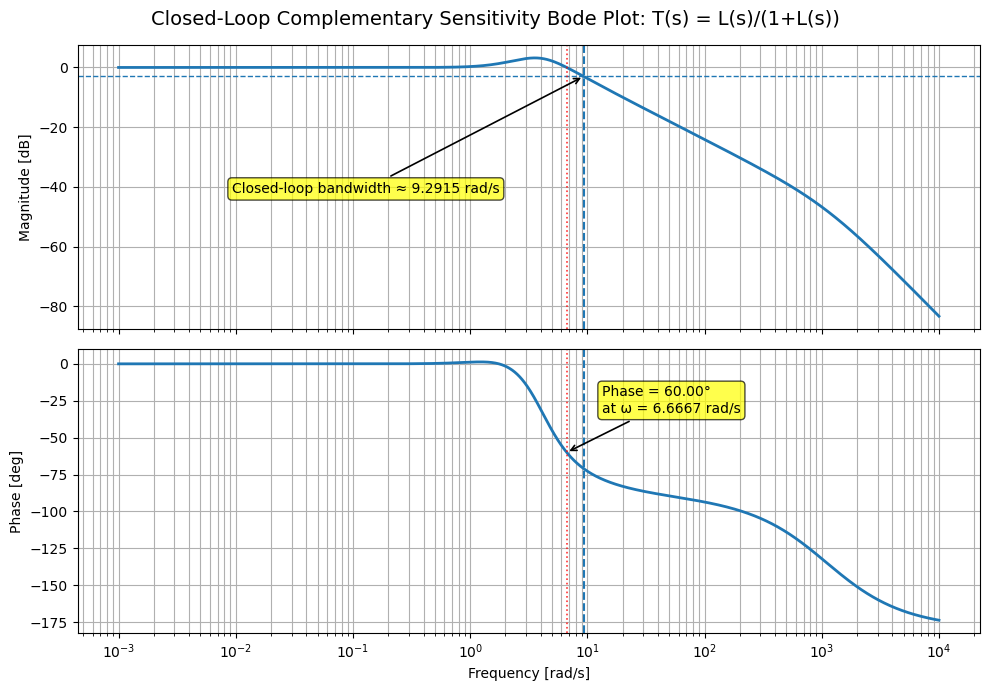
Sensitivity Bode Plot
# ============================================================
# Closed-loop Bode plot to verify bandwidth
# S(s) = 1 /(1+L)
# ============================================================
ws, mags_db, phases_deg = bode_data(S, omega)

fig, ax = plt.subplots(2, 1, figsize=(10, 7), sharex=True)
fig.suptitle("Closed-Loop Sensitivity Bode Plot: S(s) = 1/(1+L(s))", fontsize=14)

ax[0].semilogx(ws, mags_db, linewidth=2)
ax[0].axhline(-3, linestyle='--', linewidth=1)
ax[0].set_ylabel("Magnitude [dB]")
ax[0].grid(True, which='both')

ax[1].semilogx(ws, phases_deg, linewidth=2)
ax[1].set_ylabel("Phase [deg]")
ax[1].set_xlabel("Frequency [rad/s]")
ax[1].grid(True, which='both')

if np.isfinite(bw_closed) and bw_closed > 0:
    for axes in ax:
        axes.axvline(bw_closed, linestyle='--', linewidth=1.5)

    ax[0].annotate(rf'Closed-loop bandwidth $\approx$ {bw_closed:.4f} rad/s',
                   xy=(bw_closed, np.interp(bw_closed, wt, magt_db)),
                   xytext=(bw_closed/1000, np.interp(bw_closed, wt, magt_db)-40),
                   arrowprops=dict(arrowstyle='->', color='black', lw=1.2),
                   ha='left', va='bottom', fontsize=10, bbox=dict(boxstyle="round,pad=0.3", fc="yellow", alpha=0.7))

# ====================== Phase Annotation ======================
if np.isfinite(pm) and pm > 0 and np.isfinite(wp) and wp > 0:
    # Find the phase value on the plotted curve at ω = wp (phase crossover)
    phase_at_wp = np.interp(wp, wt, phaset_deg)

    ax[1].annotate(f'Phase = {pm:.2f}°\nat ω = {wp:.4f} rad/s',
                   xy=(wp, phase_at_wp),                    # point on the curve
                   xytext=(wp * 2.0, phase_at_wp + 25),     # text position: right and above
                   arrowprops=dict(arrowstyle='->', color='black', lw=1.2),
                   ha='left', va='bottom', fontsize=10, bbox=dict(boxstyle="round,pad=0.3", fc="yellow", alpha=0.7))

    # Optional: add vertical line at phase crossover frequency
    for axes in ax:
        axes.axvline(wp, linestyle=':', linewidth=1.2, color='red', alpha=0.8)

plt.tight_layout()
plt.show()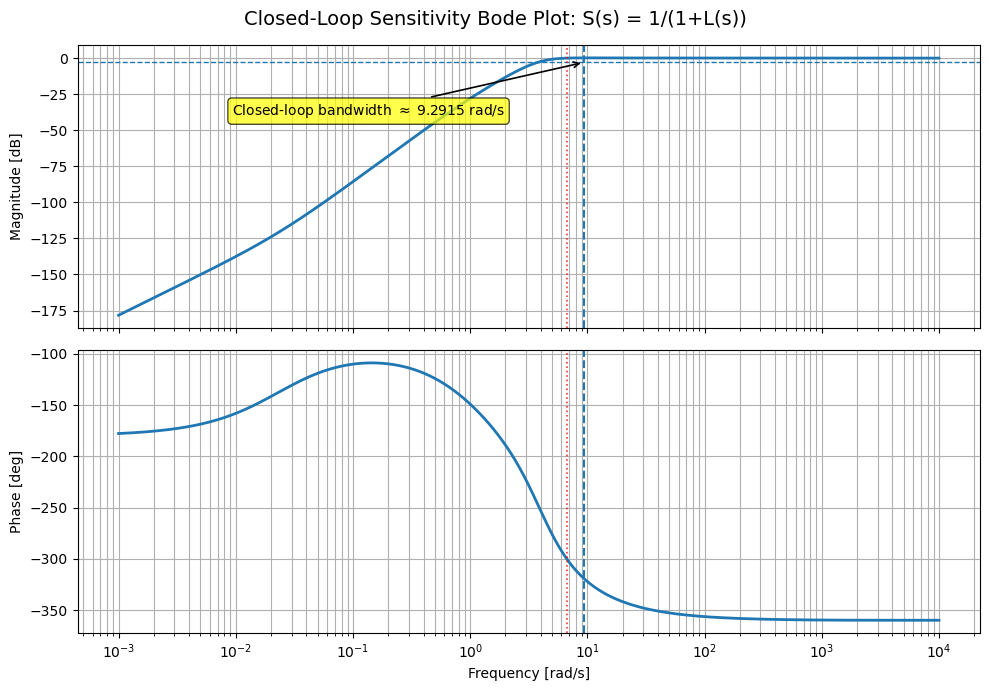
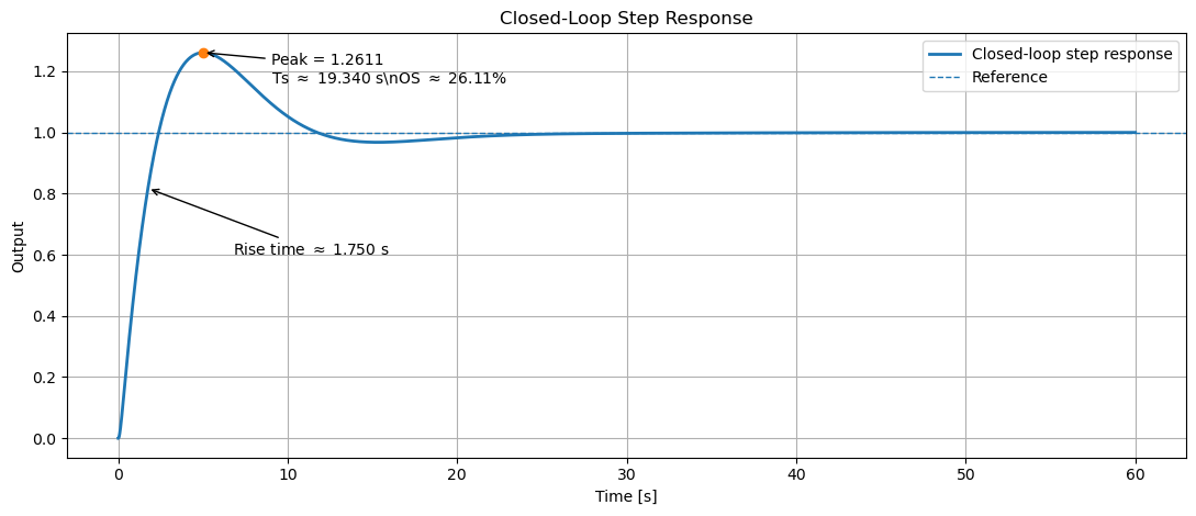
Plot Closed Loop Step Response
# ============================================================
# Closed-loop step response
# ============================================================
t_cl = np.linspace(0, 5, 3000)
t3, y3 = ct.step_response(T, T=t_cl)

info = ct.step_info(T)

plt.figure(figsize=(10, 4.5))
plt.plot(t3, y3, linewidth=2)
plt.axhline(1, linestyle='--', linewidth=1)
plt.title("Closed-Loop Step Response")
plt.xlabel("Time [s]")
plt.ylim(0, 1.4)
plt.ylabel("Output")
plt.grid(True)

peak_idx = np.argmax(y3)
plt.plot(t3[peak_idx], y3[peak_idx], 'o')
plt.annotate(rf"Peak = {y3[peak_idx]:.4f}\nTsettling $\approx$ {info['SettlingTime']:.4f} s",
             xy=(t3[peak_idx], y3[peak_idx]),
             xytext=(t3[peak_idx] + 0.5
                     , y3[peak_idx] - 0.15),
             arrowprops=dict(arrowstyle='->'))

plt.show()

print("\n================ STEP INFO FOR CLOSED LOOP ================\n")
for k, v in info.items():
    print(f"{k:20s}: {v}")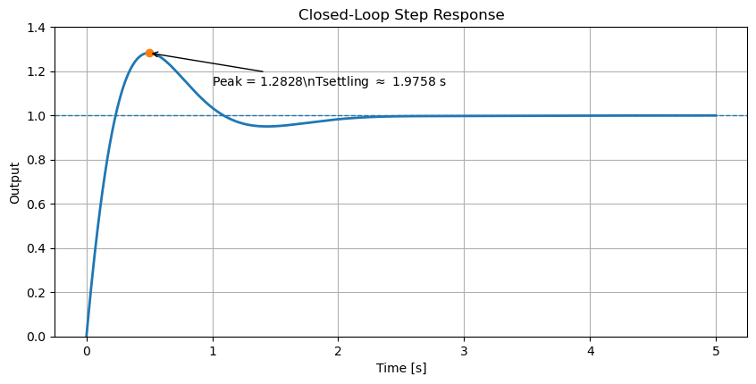
================ STEP INFO FOR CLOSED LOOP ================

RiseTime            : 0.16464658424747655
SettlingTime        : 1.9757590109697185
SettlingMin         : 0.9500992854912289
SettlingMax         : 1.2827329688449818
Overshoot           : 28.273296884498148
Undershoot          : 0.0
Peak                : 1.2827329688449818
PeakTime            : 0.4939397527424296
SteadyStateValue    : 1.0000000000000002
Discretize the PID Controller
Discretize your PID controller and test it in a closed loop with the plant to verify it works. For sampling time use Ts = 0.01 sec.
Define symbols
s, z = sp.symbols('s z')
K_sym, a, tau, Ts = sp.symbols('K a tau T_s', positive=True, real=True)
Define the Continuous-Time Controller
# C(s) = K (s+a)^2 / [ s (tau s + 1) ]

C_s = K_sym * (s + a)**2 / (s * (tau*s + 1))

display(Eq(sp.Symbol('C(s)'), C_s))Expand Numerator for Clarity
C_s_expanded = sp.simplify(K_sym * (s**2 + 2*a*s + a**2) / (s * (tau*s + 1)))
display(Eq(sp.Symbol('C(s)'), C_s_expanded))Tustin Substitution
# s -> (2/Ts) * (z-1)/(z+1)

s_tustin = (sp.Integer(2) / Ts) * ((z - 1) / (z + 1))

display(Eq(sp.Symbol(r's_{\text{Tustin}}'), s_tustin))Substitute into 
C_z_sub = sp.simplify(C_s.subs(s, s_tustin))
display(Eq(sp.Symbol('C(z)'), C_z_sub))Introduce 
q = sp.symbols('q')

C_q = sp.simplify(C_s.subs(s, (sp.Integer(2)/Ts) * q))
display(Eq(sp.Symbol('q'), (z - 1)/(z + 1)))
display(Eq(sp.Symbol('C(q)'), C_q))Substitute Numerical Values Used in the Lab
# K = 71.699528, a = 1.7777, tau = 0.0009, Ts = 0.01

vals = {
    K_sym: sp.Float('71.699528'),
    a: sp.Float('1.7777'),
    tau: sp.Float('0.0009'),
    Ts: sp.Float('0.01')
}

C_q_num = sp.simplify(C_q.subs(vals))
display(Eq(sp.Symbol('C(q)'), C_q_num))Expand the Tustin Scaling Terms
# 2/Ts = 200, tau*(2/Ts) = 0.18

two_over_Ts = sp.simplify((sp.Integer(2)/Ts).subs(vals))
tau_two_over_Ts = sp.simplify((tau * (sp.Integer(2)/Ts)).subs(vals))display(Eq(sp.Symbol(r'2/T_s'), two_over_Ts))
display(Eq(sp.Symbol(r'2\tau/T_s'), tau_two_over_Ts))C_q_num_manual = sp.Float('71.699528') * (sp.Float('200')*q + sp.Float('1.7777'))**2 / (
sp.Float('200')*q * (sp.Float('0.18')*q + 1)
)
display(Eq(sp.Symbol('C(q)'), sp.simplify(C_q_num_manual)))Replace 
C_z = sp.simplify(C_q_num_manual.subs(q, (z - 1)/(z + 1)))
display(Eq(sp.Symbol('C(z)'), C_z))Show Intermediate Steps
term1 = sp.simplify((sp.Float('200')*q + sp.Float('1.7777')).subs(q, (z - 1)/(z + 1)))
term2 = sp.simplify((sp.Float('0.18')*q + 1).subs(q, (z - 1)/(z + 1)))
term3 = sp.simplify((sp.Float('200')*q).subs(q, (z - 1)/(z + 1)))

display(Eq(sp.Symbol(r'200q + 1.7777'), term1))
display(Eq(sp.Symbol(r'0.18q + 1'), term2))
display(Eq(sp.Symbol(r'200q'), term3))Write as a Rational Function in 
C_z_together = sp.together(C_z)
display(Eq(sp.Symbol('C(z)'), C_z_together))Expand the Numerator and Denominator
num_z, den_z = sp.fraction(C_z_together)
num_z = sp.expand(num_z)
den_z = sp.expand(den_z)

display(Eq(sp.Symbol('Numerator\; in\; z'), num_z))
display(Eq(sp.Symbol('Denominator\; in\; z'), den_z))Normalize Denominator Leading Coefficient
den_poly = sp.Poly(den_z, z)
lead_coeff = den_poly.LC()

num_z_norm = sp.expand(num_z / lead_coeff)
den_z_norm = sp.expand(den_z / lead_coeff)

display(Eq(sp.Symbol('Leading\; denominator\; coefficient'), lead_coeff))
display(Eq(sp.Symbol('Normalized\; numerator'), num_z_norm))
display(Eq(sp.Symbol('Normalized\; denominator'), den_z_norm))Convert to Form
# Divide numerator and denominator by z^2
num_zinv = sp.expand(num_z_norm / z**2)
den_zinv = sp.expand(den_z_norm / z**2)

display(Eq(sp.Symbol('Numerator\; in\; z^{-1}\; form'), num_zinv))
display(Eq(sp.Symbol('Denominator\; in\; z^{-1}\; form'), den_zinv))Discrete Transfer Function Form
C_zinv = sp.simplify(num_zinv / den_zinv)
display(Eq(sp.Symbol('C(z)'), C_zinv))Results Summary
print("\n================ CONTINUOUS CONTROLLER ================\n")
display(C_s)

print("\n================ TUSTIN SUBSTITUTION ================\n")
display(s_tustin)

print("\n================ DISCRETE CONTROLLER C(z) ================\n")
display(C_z_together)

print("\n================ NORMALIZED FORM IN z ================\n")
print("Numerator:")
display(num_z_norm)
print("\nDenominator:")
display(den_z_norm)

print("\n================ z^{-1} FORM ================\n")
print("Numerator:")
display(num_zinv)
print("\nDenominator:")
display(den_zinv)

print("\n================ DISCRETE CONTRROLLER TF FORM ================\n")
display(C_zinv)
================ CONTINUOUS CONTROLLER ================
================ TUSTIN SUBSTITUTION ================
================ DISCRETE CONTROLLER C(z) ================
================ NORMALIZED FORM IN z ================

Numerator:
Denominator:
================ z^{-1} FORM ================

Numerator:
Denominator:
================ DISCRETE CONTRROLLER TF FORM ================
Verify with Python Control System Library
Define Continuous Time Controller
# C(s) = K (s+a)^2 / [ s (tau*s + 1) ]

K = 71.699528
a = 1.7777
tau = 0.0009
Ts = 0.01

s = ct.tf('s')

C_s = K * (s + a)**2 / (s * (tau*s + 1))

print("\n================ CONTINUOUS-TIME CONTROLLER C(s) ================\n")
C_s
================ CONTINUOUS-TIME CONTROLLER C(s) ================
Discretize using Tustin
# In python-control, 'tustin' and 'bilinear' are supported.

C_z_tustin = ct.c2d(C_s, Ts, method='tustin')

print("\n================ DISCRETE-TIME CONTROLLER C(z) VIA TUSTIN ================\n")
C_z_tustin
================ DISCRETE-TIME CONTROLLER C(z) VIA TUSTIN ================
w_gc = 10 / 1.5   # ~6.6667 rad/s

C_z_prewarp = ct.c2d(C_s, Ts, method='tustin', prewarp_frequency=w_gc)

print("\n================ TUSTIN WITH PREWARP ================\n")
C_z_prewarp
================ TUSTIN WITH PREWARP ================
Get Numerator and Denominator Coefficients
num = np.squeeze(C_z_tustin.num[0][0])
den = np.squeeze(C_z_tustin.den[0][0])

print("\nNumerator coefficients:")
num
Numerator coefficients:
array([ 12369.45680703, -24303.00452468, 11937.38815982])print("\nDenominator coefficients:")
den
Denominator coefficients:
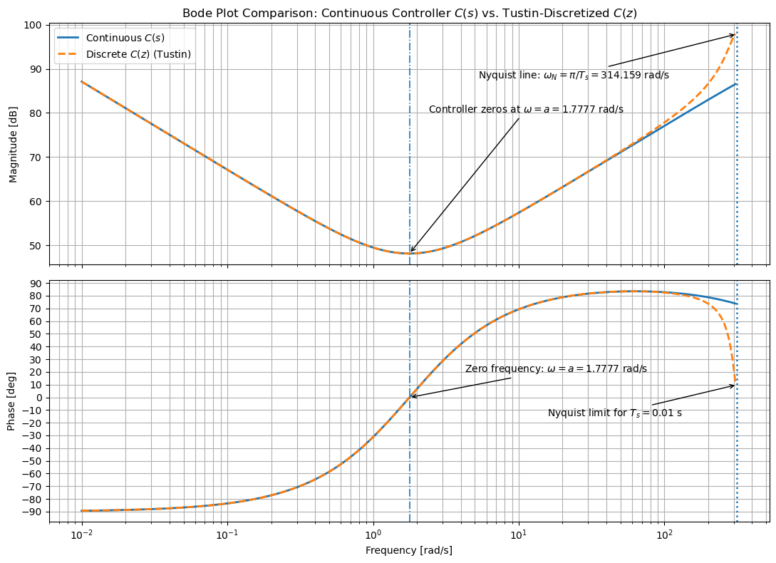
array([ 1. , -0.30508475, -0.69491525])Bode Plots of and 
# ============================================================
# Controller parameters
# ============================================================
K = 71.699528
a = 1.7777
tau = 0.0009
Ts = 0.01

# ============================================================
# Define continuous-time controller C(s)
# C(s) = K (s+a)^2 / [ s (tau*s + 1) ]
# ============================================================
s = ct.tf('s')
C_s = K * (s + a)**2 / (s * (tau*s + 1))

# ============================================================
# Discretize with Tustin to get C(z)
# ============================================================
C_z = ct.c2d(C_s, Ts, method='tustin')

print("Continuous-time controller C(s):")
display(C_s)

print("\nDiscrete-time controller C(z) via Tustin:")
display(C_z)

# ============================================================
# Frequency range
# For comparison, only plot up to a bit below Nyquist
# ============================================================
w_nyq = np.pi / Ts                    # Nyquist frequency [rad/s]
w_min = 1e-2
w_max = 0.98 * w_nyq
omega = np.logspace(np.log10(w_min), np.log10(w_max), 3000)

# ============================================================
# Frequency responses
# Use the same omega grid for both C(s) and C(z)
# ============================================================
mag_s, phase_s, omega_s = ct.frequency_response(C_s, omega)
mag_z, phase_z, omega_z = ct.frequency_response(C_z, omega)

mag_s = np.squeeze(mag_s)
mag_z = np.squeeze(mag_z)

# unwrap phase so both curves are readable
phase_s_deg = np.degrees(np.unwrap(np.squeeze(phase_s)))
phase_z_deg = np.degrees(np.unwrap(np.squeeze(phase_z)))

mag_s_db = 20 * np.log10(mag_s)
mag_z_db = 20 * np.log10(mag_z)

# ============================================================
# Useful frequencies for annotations
# ============================================================
w_zero = a
w_pseudo = 1 / tau

# helper for interpolation in log-frequency domain
def interp_logx(x, xp, fp):
    return np.interp(np.log10(x), np.log10(xp), fp)

# values for annotations
mag_s_zero = interp_logx(w_zero, omega, mag_s_db)
mag_s_pseudo = interp_logx(min(w_pseudo, omega[-1]), omega, mag_s_db)

phase_s_zero = interp_logx(w_zero, omega, phase_s_deg)
phase_s_pseudo = interp_logx(min(w_pseudo, omega[-1]), omega, phase_s_deg)

# ============================================================
# Plot
# ============================================================
fig, ax = plt.subplots(2, 1, figsize=(11, 8), sharex=True)

# ---------------- Magnitude ----------------
ax[0].semilogx(omega, mag_s_db, linewidth=2, label=r'Continuous $C(s)$')
ax[0].semilogx(omega, mag_z_db, linewidth=2, linestyle='--', label=r'Discrete $C(z)$ (Tustin)')

ax[0].axvline(w_nyq, linestyle=':', linewidth=1.8)
ax[0].axvline(w_zero, linestyle='-.', linewidth=1.2)
if w_pseudo < omega[-1]:
    ax[0].axvline(w_pseudo, linestyle='-.', linewidth=1.2)

ax[0].set_ylabel('Magnitude [dB]')
ax[0].set_title('Bode Plot Comparison: Continuous Controller $C(s)$ vs. Tustin-Discretized $C(z)$')
ax[0].grid(True, which='both')
ax[0].legend()

ax[0].annotate(
    rf'Controller zeros at $\omega=a={w_zero:.4f}$ rad/s',
    xy=(w_zero, mag_s_zero),
    xytext=(w_zero * 1.35, mag_s_zero + 32),
    arrowprops=dict(arrowstyle='->')
)

if w_pseudo < omega[-1]:
    ax[0].annotate(
        rf'Pseudo-pole at $\omega=1/\tau={w_pseudo:.1f}$ rad/s',
        xy=(w_pseudo, mag_s_pseudo),
        xytext=(w_pseudo / 5, mag_s_pseudo - 18),
        arrowprops=dict(arrowstyle='->')
    )

ax[0].annotate(
    rf'Nyquist line: $\omega_N=\pi/T_s={w_nyq:.3f}$ rad/s',
    xy=(w_nyq, interp_logx(w_nyq * 0.98, omega, mag_z_db)),
    xytext=(w_nyq / 60, interp_logx(w_nyq * 0.98, omega, mag_z_db) - 10),
    arrowprops=dict(arrowstyle='->')
)

# ---------------- Phase ----------------
ax[1].semilogx(omega, phase_s_deg, linewidth=2, label=r'Continuous $C(s)$')
ax[1].semilogx(omega, phase_z_deg, linewidth=2, linestyle='--', label=r'Discrete $C(z)$ (Tustin)')

ax[1].axvline(w_nyq, linestyle=':', linewidth=1.8)
ax[1].axvline(w_zero, linestyle='-.', linewidth=1.2)
if w_pseudo < omega[-1]:
    ax[1].axvline(w_pseudo, linestyle='-.', linewidth=1.2)

ax[1].set_xlabel('Frequency [rad/s]')
ax[1].set_ylabel('Phase [deg]')
ax[1].grid(True, which='both')

# more phase tick marks
phase_min = min(np.nanmin(phase_s_deg), np.nanmin(phase_z_deg))
phase_max = max(np.nanmax(phase_s_deg), np.nanmax(phase_z_deg))
yt_lo = 10 * np.floor(phase_min / 10)
yt_hi = 10 * np.ceil(phase_max / 10)
ax[1].set_yticks(np.arange(yt_lo, yt_hi + 10, 10))

ax[1].annotate(
    rf'Zero frequency: $\omega=a={w_zero:.4f}$ rad/s',
    xy=(w_zero, phase_s_zero),
    xytext=(w_zero * 2.4, phase_s_zero + 20),
    arrowprops=dict(arrowstyle='->')
)

if w_pseudo < omega[-1]:
    ax[1].annotate(
        rf'Pseudo-pole: $\omega=1/\tau={w_pseudo:.1f}$ rad/s',
        xy=(w_pseudo, phase_s_pseudo),
        xytext=(w_pseudo / 6, phase_s_pseudo - 35),
        arrowprops=dict(arrowstyle='->')
    )

ax[1].annotate(
    rf'Nyquist limit for $T_s={Ts}$ s',
    xy=(w_nyq, interp_logx(w_nyq * 0.98, omega, phase_z_deg)),
    xytext=(w_nyq / 20, interp_logx(w_nyq * 0.98, omega, phase_z_deg) - 25),
    arrowprops=dict(arrowstyle='->')
)

plt.tight_layout()
plt.show()
Continuous-time controller C(s):
Discrete-time controller C(z) via Tustin:
Parallel PID Discretization using Tustin / Bilinear Transform
Define Symbols
s, z = sp.symbols('s z', complex=True)
K, a, tau, Ts = sp.symbols('K a tau T_s', positive=True, real=True)

# Parallel PID symbols
kp, ki, kd, N = sp.symbols('k_p k_i k_d N', real=True)
Controller Transfer Function 
# C(s) = K (s+a)^2 / [ s (tau s + 1) ]

C_s = sp.simplify(K * (s + a)**2 / (s * (tau*s + 1)))
display(Eq(sp.Symbol('C(s)'), C_s))Expand Numberator of 
C_s_expanded = sp.simplify(K * (s**2 + 2*a*s + a**2) / (s * (tau*s + 1)))
display(Eq(sp.Symbol('C(s)'), C_s_expanded))Write Continuous Controller Transfer Function in Filtered Parallel PID Form
# C(s) = kp + ki/s + kd * (N s)/(s+N)

C_parallel_s = kp + ki/s + kd * (N*s)/(s + N)
display(Eq(sp.Symbol('C_{parallel}(s)'), C_parallel_s))Put Filtered Parallel PID Form over Common Denominator
C_parallel_common = sp.simplify(sp.together(C_parallel_s))
display(Eq(sp.Symbol('C_{parallel}(s)'), C_parallel_common))Isolate Numerator and Denominator
num_par, den_par = sp.fraction(C_parallel_common)
num_par = sp.expand(num_par)
den_par = sp.expand(den_par)

display(Eq(sp.Symbol('Numerator_{parallel}(s)'), num_par))
display(Eq(sp.Symbol('Denominator_{parallel}(s)'), den_par))Setup Coefficient Matching
# Continuous controller:
# C(s) = K(s+a)^2 / [s(tau*s + 1)]
#
# Parallel filtered PID:
# C(s) = kp + ki/s + kd*(N*s)/(s+N), with N = 1/tau

C_parallel_tau = sp.simplify(C_parallel_s.subs(N, 1/tau))
display(Eq(sp.Symbol('C_{parallel}(s)'), C_parallel_tau))C_parallel_tau_common = sp.simplify(sp.together(C_parallel_tau))
display(Eq(sp.Symbol('C_{parallel}(s)'), C_parallel_tau_common))num_tau, den_tau = sp.fraction(C_parallel_tau_common)
num_tau = sp.expand(num_tau)
den_tau = sp.expand(den_tau)
display(Eq(sp.Symbol('Numerator_{parallel}(s)'), num_tau))
display(Eq(sp.Symbol('Denominator_{parallel}(s)'), den_tau))target_num = sp.expand(K * (s + a)**2)
display(Eq(sp.Symbol('Targe\; numerator'), target_num))Collect Coefficients in 
poly_num_tau = sp.Poly(num_tau, s)
poly_target = sp.Poly(target_num, s)

display(sp.Symbol('Parallel\; coeffs'),sp.Matrix(poly_num_tau.all_coeffs()))
display(sp.Symbol('Target\; coeffs'), sp.Matrix(poly_target.all_coeffs()))Perform Coefficient Matching
coeff_eqs = [
    sp.Eq(poly_num_tau.all_coeffs()[0], poly_target.all_coeffs()[0]),  # s^2
    sp.Eq(poly_num_tau.all_coeffs()[1], poly_target.all_coeffs()[1]),  # s^1
    sp.Eq(poly_num_tau.all_coeffs()[2], poly_target.all_coeffs()[2]),  # s^0
]

sol_pid = sp.solve(coeff_eqs, (kp, ki, kd), dict=True)[0]

kp_expr = sp.simplify(sol_pid[kp])
ki_expr = sp.simplify(sol_pid[ki])
kd_expr = sp.simplify(sol_pid[kd])

display(Eq(kp, kp_expr))
display(Eq(ki, ki_expr))
display(Eq(kd, kd_expr))Perform Tustin Substitution
# s -> (2/Ts) * (z-1)/(z+1)

s_tustin = sp.simplify((sp.Integer(2)/Ts) * (z - 1)/(z + 1))
display(Eq(sp.Symbol(r's_{Tustin}'), s_tustin))Perform Tustin Substitution for Proportional Branch
C_P_z = kp_expr
display(Eq(sp.Symbol('C_{P}(z)'), C_P_z))Perform Tustin Substitution for Integral Branch
C_I_s = ki_expr / s
display(Eq(sp.Symbol('C_{I}(s)'), C_I_s))

C_I_z = sp.simplify(C_I_s.subs(s, s_tustin))
display(Eq(sp.Symbol('C_{I}(z)'), C_I_z))# Show the standard closed form
C_I_z_closed = sp.simplify(ki_expr * (Ts/sp.Integer(2)) * (z + 1)/(z - 1))
display(Eq(sp.Symbol('C_{I}(z)'), C_I_z_closed))Perform Tustin Substitution for Derivative Branch
C_D_s = kd_expr * ((1/tau) * s) / (s + 1/tau)
display(Eq(sp.Symbol('C_{D}(s)'), C_D_s))C_D_z = sp.simplify(C_D_s.subs(s, s_tustin))
display(Eq(sp.Symbol('C_{D}(z)'), C_D_z))Simplify the Derivative Branch into Standard Rational Form
C_D_z_together = sp.simplify(sp.together(C_D_z))
display(Eq(sp.Symbol('C_D(z)'), C_D_z_together))

num_Dz, den_Dz = sp.fraction(C_D_z_together)
num_Dz = sp.expand(num_Dz)
den_Dz = sp.expand(den_Dz)

display(Eq(sp.Symbol('Numerator_{D}(z)'), num_Dz))
display(Eq(sp.Symbol('Denominator_{D}(z)'), den_Dz))Assemble the Exact Tustin Parallel PID
C_parallel_z = sp.simplify(C_P_z + C_I_z_closed + C_D_z_together)
display(Eq(sp.Symbol('C_{parallel,Tustin}(z)'), C_parallel_z))

# Show the branch sum explicitly
display(Eq(sp.Symbol('C(z)'), sp.Symbol('C_P(z)') + sp.Symbol('C_I(z)') + sp.Symbol('C_D(z)')))Verify Correctness of Controller Discretization
C_full_tustin = sp.simplify(C_s.subs(s, s_tustin))
display(Eq(sp.Symbol('C_{full,Tustin}(z)'), C_full_tustin))# Difference should be zero for exact Tustin-based parallel realization
verification = sp.simplify(sp.together(C_parallel_z - C_full_tustin))
display(Eq(sp.Symbol('C_{parallel,Tustin}(z) - C_{full,Tustin}(z)'), verification))Substitute Numerical Values
vals = {
    K: sp.Float('71.699528'),
    a: sp.Float('1.7777'),
    tau: sp.Float('0.0009'),
    Ts: sp.Float('0.01'),
}
kp_num = sp.N(kp_expr.subs(vals))
ki_num = sp.N(ki_expr.subs(vals))
kd_num = sp.N(kd_expr.subs(vals))
N_num = sp.N((1/tau).subs(vals))
C_P_num = sp.N(C_P_z.subs(vals))
C_I_num = sp.simplify(C_I_z_closed.subs(vals))
C_D_num = sp.simplify(C_D_z_together.subs(vals))
C_total_num = sp.simplify(C_parallel_z.subs(vals))
display(Eq(kp, kp_num))
display(Eq(ki, ki_num))
display(Eq(kd, kd_num))
display(Eq(N, N_num))
display(Eq(sp.Symbol('C_P(z)'), C_P_num))
display(Eq(sp.Symbol('C_I(z)'), C_I_num))
display(Eq(sp.Symbol('C_D(z)'), C_D_num))
display(Eq(sp.Symbol('C(z)'), C_total_num))Summary of Results
print("\n================ CONTINUOUS CONTROLLER =================\n")
display(C_s)

print("\n================ CONTINUOUS PARALLEL PID MATCH =================\n")
print("kp =")
display(kp_expr)
print("\nki =")
display(ki_expr)
print("\nkd =")
display(kd_expr)
print("\nN = 1/tau")

print("\n================ EXACT TUSTIN-BASED PARALLEL BRANCHES =================\n")
print("C_P(z) =")
display(C_P_z)

print("\nC_I(z) =")
display(C_I_z_closed)

print("\nC_D(z) =")
display(C_D_z_together)

print("\n================ NUMERICAL VALUES =================\n")
print(f"kp = {kp_num}")
print(f"ki = {ki_num}")
print(f"kd = {kd_num}")
print(f"N  = {N_num}")

print("\nC_P(z) =")
display(C_P_num)

print("\nC_I(z) =")
display(C_I_num)

print("\nC_D(z) =")
display(C_D_num)

print("\nVerification C_parallel,Tustin(z) - C_full,Tustin(z) =")
display(verification)
================ CONTINUOUS CONTROLLER =================
================ CONTINUOUS PARALLEL PID MATCH =================

kp =
ki =
kd =
N = 1/tau

================ EXACT TUSTIN-BASED PARALLEL BRANCHES =================

C_P(z) =
C_I(z) =
C_D(z) =
================ NUMERICAL VALUES =================

kp = 254.716574371937
ki = 226.586088070439
kd = 71.4702830830653
N  = 1111.11111111111

C_P(z) =
C_I(z) =
C_D(z) =
Verification C_parallel,Tustin(z) - C_full,Tustin(z) =
Verify with Control Systems Library
Continuous Time Controller Parameters
K = 71.699528
a = 1.7777
tau = 0.0009
Ts = 0.01

print("\n================ GIVEN PARAMETERS ================\n")
print(f"K   = {K}")
print(f"a   = {a}")
print(f"tau = {tau}")
print(f"Ts  = {Ts}")
================ GIVEN PARAMETERS ================

K   = 71.699528
a   = 1.7777
tau = 0.0009
Ts  = 0.01
# Laplace and z variables
s = ct.tf('s')
z = ct.tf('z')
Define the Continuous-Time Controller
# C(s) = K (s+a)^2 / [ s (tau*s + 1) ]

C_s = K * (s + a)**2 / (s * (tau*s + 1))

print("\n================ ORIGINAL CONTINUOUS CONTROLLER ================\n")
print("C(s) =")
C_s
================ ORIGINAL CONTINUOUS CONTROLLER ================

C(s) =
Convert into Continuous Parallel Fitered PID Form
# Desired form:
#   C(s) = kp + ki/s + kd * (N*s)/(s+N)
# where
#   N = 1/tau
#
# Matching gives:
#   ki = K a^2
#   kp = 2 K a - ki tau
#   kd = K - kp tau
# ============================================================
N = 1 / tau
ki = K * a**2
kp = 2 * K * a - ki * tau
kd = K - kp * tau

print("\n================ CONTINUOUS PARALLEL PID PARAMETERS ================\n")
print(f"N  = 1/tau = {N:.10f}")
print(f"ki = K*a^2 = {ki:.10f}")
print(f"kp = 2*K*a - ki*tau = {kp:.10f}")
print(f"kd = K - kp*tau = {kd:.10f}")
================ CONTINUOUS PARALLEL PID PARAMETERS ================

N  = 1/tau = 1111.1111111111
ki = K*a^2 = 226.5860880704
kp = 2*K*a - ki*tau = 254.7165743719
kd = K - kp*tau = 71.4702830831
Build the Continuous Parallel Branches
C_P_s = ct.tf([kp], [1])
C_I_s = ct.tf([ki], [1, 0])          # ki / s
C_D_s = kd * ct.tf([N, 0], [1, N])   # kd * (N s)/(s + N)

C_parallel_s = ct.minreal(C_P_s + C_I_s + C_D_s, verbose=False)
print("\nContinuous proportional branch C_P(s) =")
C_P_s
Continuous proportional branch C_P(s) =
print("\nContinuous integral branch C_I(s) =")
C_I_s
Continuous integral branch C_I(s) =
print("\nContinuous derivative branch C_D(s) =")
C_D_s
Continuous derivative branch C_D(s) =
print("\nSum of continuous parallel branches C_parallel(s) =")
C_parallel_s
Sum of continuous parallel branches C_parallel(s) =
Verify Continuous Equality between and 
C_cont_err = ct.minreal(C_parallel_s - C_s, verbose=False)
print("\nContinuous verification: C_parallel(s) - C(s) =")
C_cont_err
Continuous verification: C_parallel(s) - C(s) =
Note: above result is practically zero. Discrepancy due to roundoff error.
Discretize Each Branch with Tustin
# Exact Tustin-based parallel realization means:
#   C_P(z) = Tustin{kp}
#   C_I(z) = Tustin{ki/s}
#   C_D(z) = Tustin{kd * (N s)/(s+N)}
#
# Then:
#   C_parallel_Tustin(z) = C_P(z) + C_I(z) + C_D(z)
# ============================================================
C_P_z = ct.c2d(C_P_s, Ts, method='tustin')
C_I_z = ct.c2d(C_I_s, Ts, method='tustin')
C_D_z = ct.c2d(C_D_s, Ts, method='tustin')

C_parallel_z = ct.minreal(C_P_z + C_I_z + C_D_z, verbose=False)
print("\n================ TUSTIN-DISCRETIZED BRANCHES ================\n")
print("C_P(z) =")
C_P_z
================ TUSTIN-DISCRETIZED BRANCHES ================

C_P(z) =
print("\nC_I(z) =")
C_I_z
C_I(z) =
print("\nC_D(z) =")
C_D_z
C_D(z) =
print("\nSum of Tustin-discretized branches C_parallel_Tustin(z) =")
C_parallel_z
Sum of Tustin-discretized branches C_parallel_Tustin(z) =
Discretize the Full Controller with Tustin
C_full_tustin_z = ct.c2d(C_s, Ts, method='tustin')

print("\n================ FULL-CONTROLLER TUSTIN DISCRETIZATION ================\n")
print("C_full_Tustin(z) =")
C_full_tustin_z
================ FULL-CONTROLLER TUSTIN DISCRETIZATION ================

C_full_Tustin(z) =
Verify Exact Equality between and 
# For an exact Tustin-based parallel realization, these should match.

C_disc_err = ct.minreal(C_parallel_z - C_full_tustin_z, verbose=False)

print("\n================ STEP 6: VERIFICATION ================\n")
print("C_parallel_Tustin(z) - C_full_Tustin(z) =")
C_disc_err
================ STEP 6: VERIFICATION ================

C_parallel_Tustin(z) - C_full_Tustin(z) =
Note: above result is practically zero. Discrepancy due to roundoff error.
Extract Coefficients for Each Discrete Branch
def print_tf_coeffs(name, sys):
    num = np.squeeze(sys.num[0][0])
    den = np.squeeze(sys.den[0][0])
    print(f"\n{name}:")
    display(sys)
    print("Numerator coefficients:", num)
    print("Denominator coefficients:", den)

print("\n================ DISCRETE BRANCH COEFFICIENTS ================\n")
print_tf_coeffs("C_P(z)", C_P_z)
print_tf_coeffs("C_I(z)", C_I_z)
print_tf_coeffs("C_D(z)", C_D_z)
print_tf_coeffs("C_parallel_Tustin(z)", C_parallel_z)
================ DISCRETE BRANCH COEFFICIENTS ================


C_P(z):
Numerator coefficients: [ 254.71657437 -254.71657437]
Denominator coefficients: [ 1. -1.]

C_I(z):
Numerator coefficients: [1.13293044 1.13293044]
Denominator coefficients: [ 1. -1.]

C_D(z):
Numerator coefficients: [ 12113.60730221 -12113.60730221]
Denominator coefficients: [1.         0.69491525]

C_parallel_Tustin(z):
Numerator coefficients: [ 12369.45680703 -24303.00452472  11937.38815986]
Denominator coefficients: [ 1.         -0.30508476 -0.69491527]
Frequency Response Checks
# Compare C_parallel_Tustin(z) against C_full_Tustin(z)
# and against the continuous controller over a frequency grid.
# ============================================================
omega = np.logspace(-2, np.log10(0.98*np.pi/Ts), 2000)

# Magnitude check at a few frequencies
print("\n================ SAMPLE MAGNITUDE CHECKS ================\n")
for w in [0.1, 1.0, 5.0, 10.0, 50.0, 100.0]:
    if w < np.pi / Ts:
        val_parallel = ct.evalfr(C_parallel_z, np.exp(1j*w*Ts))
        val_full = ct.evalfr(C_full_tustin_z, np.exp(1j*w*Ts))
        print(f"omega = {w:8.3f} rad/s")
        print(f"  |C_parallel_Tustin(e^jwT)| = {abs(val_parallel):12.6f}")
        print(f"  |C_full_Tustin(e^jwT)|     = {abs(val_full):12.6f}")
================ SAMPLE MAGNITUDE CHECKS ================

omega =    0.100 rad/s
  |C_parallel_Tustin(e^jwT)| =  2273.030614
  |C_full_Tustin(e^jwT)|     =  2273.030636
omega =    1.000 rad/s
  |C_parallel_Tustin(e^jwT)| =   298.284202
  |C_full_Tustin(e^jwT)|     =   298.284205
omega =    5.000 rad/s
  |C_parallel_Tustin(e^jwT)| =   403.876027
  |C_full_Tustin(e^jwT)|     =   403.876031
omega =   10.000 rad/s
  |C_parallel_Tustin(e^jwT)| =   740.203063
  |C_full_Tustin(e^jwT)|     =   740.203070
omega =   50.000 rad/s
  |C_parallel_Tustin(e^jwT)| =  3662.149889
  |C_full_Tustin(e^jwT)|     =  3662.149922
omega =  100.000 rad/s
  |C_parallel_Tustin(e^jwT)| =  7798.386697
  |C_full_Tustin(e^jwT)|     =  7798.386768
Summary of Results
print("\n================ FINAL SUMMARY ================\n")
print("Continuous parallel filtered PID:")
print(f"  kp = {kp:.10f}")
print(f"  ki = {ki:.10f}")
print(f"  kd = {kd:.10f}")
print(f"  N  = {N:.10f}")

print("\nExact Tustin-based parallel realization:")
print("  C(z) = C_P(z) + C_I(z) + C_D(z)")
print("\nwhere")
print("  C_P(z) =")
display(C_P_z)
print("  C_I(z) =")
display(C_I_z)
print("  C_D(z) =")
display(C_D_z)
================ FINAL SUMMARY ================

Continuous parallel filtered PID:
  kp = 254.7165743719
  ki = 226.5860880704
  kd = 71.4702830831
  N  = 1111.1111111111

Exact Tustin-based parallel realization:
  C(z) = C_P(z) + C_I(z) + C_D(z)

where
  C_P(z) =
C_I(z) =
C_D(z) =
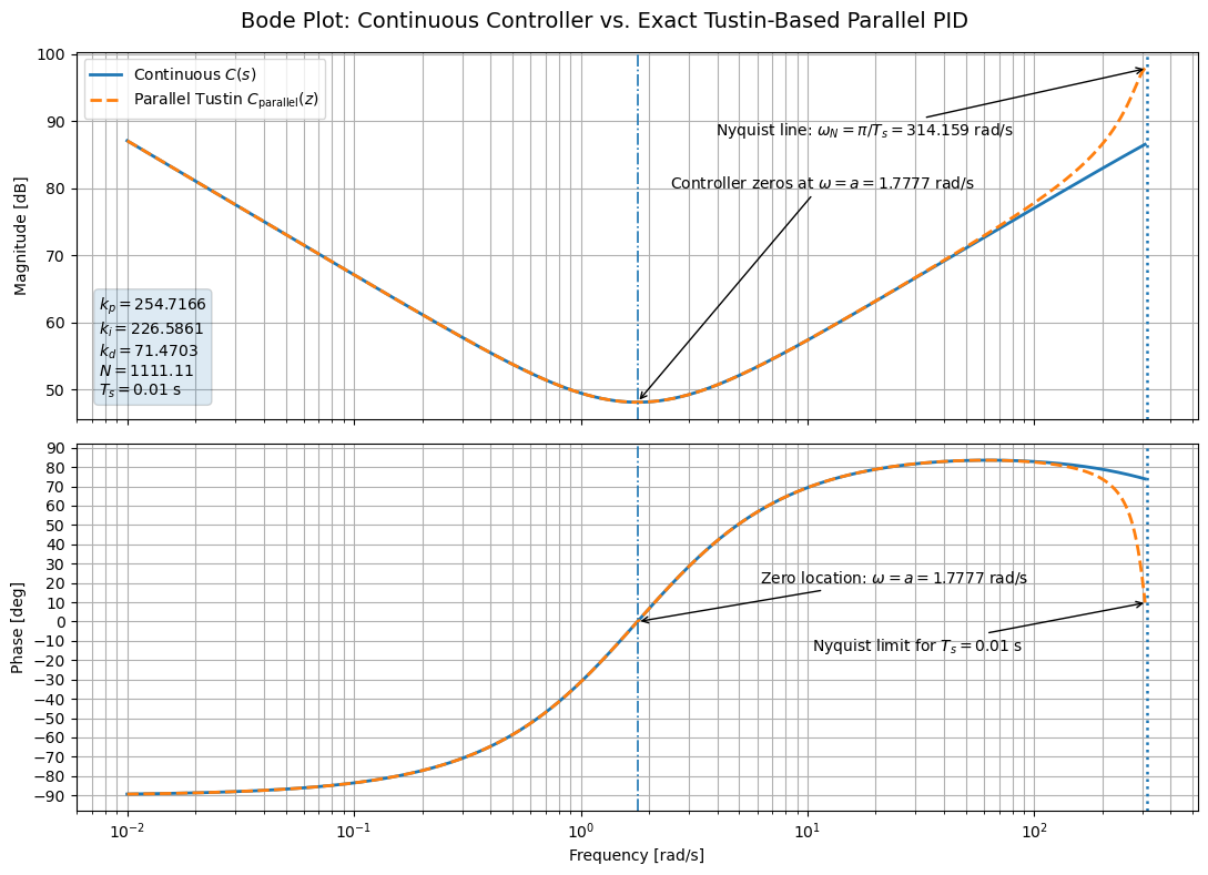
Bode Plots of and 
# ============================================================
# Controller/design parameters
# ============================================================
K = 71.699528
a = 1.7777
tau = 0.0009
Ts = 0.01

# ============================================================
# Continuous-time controller
# C(s) = K (s+a)^2 / [ s (tau*s + 1) ]
# ============================================================
s = ct.tf('s')
C_s = K * (s + a)**2 / (s * (tau*s + 1))

# ============================================================
# Continuous-time parallel filtered PID parameters
# C(s) = kp + ki/s + kd * (N s)/(s+N), N = 1/tau
# ============================================================
N = 1 / tau
ki = K * a**2
kp = 2 * K * a - ki * tau
kd = K - kp * tau

# Continuous branches
C_P_s = ct.tf([kp], [1])
C_I_s = ct.tf([ki], [1, 0])          # ki/s
C_D_s = kd * ct.tf([N, 0], [1, N])   # kd * (N s)/(s + N)

# ============================================================
# Exact Tustin-based parallel discretization
# Discretize each branch with Tustin and sum
# ============================================================
C_P_z = ct.c2d(C_P_s, Ts, method='tustin')
C_I_z = ct.c2d(C_I_s, Ts, method='tustin')
C_D_z = ct.c2d(C_D_s, Ts, method='tustin')

C_parallel_z = ct.minreal(C_P_z + C_I_z + C_D_z, verbose=False)

print("\n================ CONTINUOUS CONTROLLER =================\n")
display(C_s)

print("\n================ PARALLEL TUSTIN-DISCRETIZED CONTROLLER =================\n")
display(C_parallel_z)

# ============================================================
# Frequency range
# Only plot up to slightly below Nyquist for the discrete system
# ============================================================
w_nyq = np.pi / Ts
omega = np.logspace(-2, np.log10(0.98 * w_nyq), 3000)

# ============================================================
# Frequency-response helper
# ============================================================
def bode_data(sys, omega):
    mag, phase, omega = ct.frequency_response(sys, omega)
    mag = np.squeeze(mag)
    phase = np.squeeze(phase)

    mag_db = 20 * np.log10(mag)
    phase_deg = np.degrees(np.unwrap(phase))
    return omega, mag_db, phase_deg

omega_c, mag_c_db, phase_c_deg = bode_data(C_s, omega)
omega_d, mag_d_db, phase_d_deg = bode_data(C_parallel_z, omega)

# ============================================================
# Annotation helper
# ============================================================
def interp_logx(x, xp, fp):
    return np.interp(np.log10(x), np.log10(xp), fp)

# Frequencies of interest
w_zero = a
w_pseudo = 1 / tau

# Continuous values for annotations
mag_zero = interp_logx(w_zero, omega_c, mag_c_db)
phase_zero = interp_logx(w_zero, omega_c, phase_c_deg)

# ============================================================
# Plot
# ============================================================
fig, ax = plt.subplots(2, 1, figsize=(11, 8), sharex=True)

fig.suptitle(
    'Bode Plot: Continuous Controller vs. Exact Tustin-Based Parallel PID',
    fontsize=14
)

# ---------------- Magnitude ----------------
ax[0].semilogx(omega_c, mag_c_db, linewidth=2, label=r'Continuous $C(s)$')
ax[0].semilogx(omega_d, mag_d_db, linewidth=2, linestyle='--',
               label=r'Parallel Tustin $C_{\mathrm{parallel}}(z)$')

ax[0].set_ylabel('Magnitude [dB]')
ax[0].grid(True, which='both')
ax[0].legend()

# Nyquist line
ax[0].axvline(w_nyq, linestyle=':', linewidth=1.8)
ax[0].annotate(
    rf'Nyquist line: $\omega_N=\pi/T_s={w_nyq:.3f}$ rad/s',
    xy=(w_nyq, interp_logx(0.98*w_nyq, omega_d, mag_d_db)),
    xytext=(w_nyq/80, interp_logx(0.98*w_nyq, omega_d, mag_d_db)-10),
    arrowprops=dict(arrowstyle='->')
)

# Controller zero location
ax[0].axvline(w_zero, linestyle='-.', linewidth=1.2)
ax[0].annotate(
    rf'Controller zeros at $\omega=a={w_zero:.4f}$ rad/s',
    xy=(w_zero, mag_zero),
    xytext=(w_zero*1.4, mag_zero+32),
    arrowprops=dict(arrowstyle='->')
)

# Pseudo-pole if it lies in the plotted frequency range
if w_pseudo < omega[-1]:
    mag_pseudo = interp_logx(w_pseudo, omega_c, mag_c_db)
    ax[0].axvline(w_pseudo, linestyle='-.', linewidth=1.2)
    ax[0].annotate(
        rf'Pseudo-pole at $\omega=1/\tau={w_pseudo:.1f}$ rad/s',
        xy=(w_pseudo, mag_pseudo),
        xytext=(w_pseudo/5, mag_pseudo-18),
        arrowprops=dict(arrowstyle='->')
    )

# ---------------- Phase ----------------
ax[1].semilogx(omega_c, phase_c_deg, linewidth=2, label=r'Continuous $C(s)$')
ax[1].semilogx(omega_d, phase_d_deg, linewidth=2, linestyle='--',
               label=r'Parallel Tustin $C_{\mathrm{parallel}}(z)$')

ax[1].set_xlabel('Frequency [rad/s]')
ax[1].set_ylabel('Phase [deg]')
ax[1].grid(True, which='both')

# More phase tick labels
phase_min = min(np.min(phase_c_deg), np.min(phase_d_deg))
phase_max = max(np.max(phase_c_deg), np.max(phase_d_deg))
yt_lo = 10 * np.floor(phase_min / 10)
yt_hi = 10 * np.ceil(phase_max / 10)
ax[1].set_yticks(np.arange(yt_lo, yt_hi + 10, 10))

# Nyquist line
ax[1].axvline(w_nyq, linestyle=':', linewidth=1.8)
ax[1].annotate(
    rf'Nyquist limit for $T_s={Ts}$ s',
    xy=(w_nyq, interp_logx(0.98*w_nyq, omega_d, phase_d_deg)),
    xytext=(w_nyq/30, interp_logx(0.98*w_nyq, omega_d, phase_d_deg)-25),
    arrowprops=dict(arrowstyle='->')
)

# Zero frequency
ax[1].axvline(w_zero, linestyle='-.', linewidth=1.2)
ax[1].annotate(
    rf'Zero location: $\omega=a={w_zero:.4f}$ rad/s',
    xy=(w_zero, phase_zero),
    xytext=(w_zero*3.45, phase_zero+20),
    arrowprops=dict(arrowstyle='->')
)

# Pseudo-pole if visible
if w_pseudo < omega[-1]:
    phase_pseudo = interp_logx(w_pseudo, omega_c, phase_c_deg)
    ax[1].axvline(w_pseudo, linestyle='-.', linewidth=1.2)
    ax[1].annotate(
        rf'Pseudo-pole: $\omega=1/\tau={w_pseudo:.1f}$ rad/s',
        xy=(w_pseudo, phase_pseudo),
        xytext=(w_pseudo/2, phase_pseudo-35),
        arrowprops=dict(arrowstyle='->')
    )

# Add a small text box with PID parameters
textstr = '\n'.join((
    rf'$k_p={kp:.4f}$',
    rf'$k_i={ki:.4f}$',
    rf'$k_d={kd:.4f}$',
    rf'$N={N:.2f}$',
    rf'$T_s={Ts}$ s'
))
ax[0].text(
    0.02, 0.05, textstr,
    transform=ax[0].transAxes,
    fontsize=10,
    verticalalignment='bottom',
    bbox=dict(boxstyle='round', alpha=0.15)
)

plt.tight_layout()
plt.show()
================ CONTINUOUS CONTROLLER =================
================ PARALLEL TUSTIN-DISCRETIZED CONTROLLER =================
Add Pre-Filter to Controller Design to Prevent Noise from Causing Integrator Windup
Define Symbols and Design Constants
from IPython.display import Math

s, z = sp.symbols('s z')
K, a = sp.symbols('K a', positive=True, real=True)

# Given design parameters
BW = sp.Float('1.0')          # target closed-loop bandwidth [rad/s]
PM = sp.Float('60.0')         # desired phase margin [deg]
Ts = sp.Float('0.01')         # sample time [s]
tau = sp.Float('0.005')       # pseudo-differentiator time constant
plant_num = sp.Float('0.08681')
p1 = sp.Float('0.02397')

display(Eq(sp.Symbol(r'\omega_{BW}'), BW))
display(Eq(sp.Symbol(r'PM'), PM))
display(Eq(sp.Symbol(r'T_s'), Ts))
display(Eq(sp.Symbol(r'\tau'), tau))Define Plant , Augmented Plant and Low - Pass Filter Transfer Functions
# P(s) = 0.08681 / [s(s+0.02397)]
# f(s) = 10/(s+10)
# Pa(s) = P(s)f(s)

P = plant_num / (s * (s + p1))
f_lp = sp.Float('10.0') / (s + sp.Float('10.0'))
Pa = sp.simplify(P * f_lp)

display(Eq(sp.Symbol('P(s)'), P))
display(Eq(sp.Symbol('f(s)'), f_lp))
display(Math(r'P_{a}(s) = P(s) \times f(s)'))
display(Eq(sp.Symbol('P_{a}(s)'), Pa))Define Continuous Domain Controller Transfer Function 
# C(s) = K (s+a)^2 / [ s (tau s + 1) ]

C = sp.simplify(K * (s + a)**2 / (s * (tau*s + 1)))
display(Eq(sp.Symbol('C(s)'), C))Choose New Crossover Frequency from Bandwidth Rule
# omega_bw ~ 1.5 * omega_gc

wgc = sp.N(BW / sp.Float('1.5'))
display(Eq(sp.Symbol(r'\omega_{gc}'), wgc))Compute ZOH Phase Lag and Frequency Compensation Target
# phi_ZOH ~ (omega_gc * Ts / 2) radians

phi_zoh_rad = -wgc * Ts / 2
phi_zoh_deg = sp.N(phi_zoh_rad * 180 / sp.pi)

phase_target = sp.N(-180 + PM - phi_zoh_deg)  # compensate negative lag by adding margin allowance

display(Eq(sp.Symbol(r'\phi_{ZOH}\,[rad]'), phi_zoh_rad))
display(Eq(sp.Symbol(r'\phi_{ZOH}\,[deg]'), phi_zoh_deg))
display(Eq(sp.Symbol(r'\angle L(j\omega_{gc})\ target\ [deg]'), phase_target))Compute Open - Loop Transfer Function 
# L(s) = C(s) * Pa(s)

L = sp.simplify(C * Pa)
display(Math(r'L(s) = C(s) \times P_{a}(s)'))
display(Eq(sp.Symbol('L(s)'), L))Apply Phase Condition to Solve for 
# angle L(jw) =
#   2 atan(w/a)
#   -180
#   -atan(w/0.02397)
#   -atan(w/10)
#   -atan(w*tau)

phase_expr_deg = sp.N(
    2 * sp.atan(wgc / a) * 180 / sp.pi
    - 180
    - sp.atan(wgc / p1) * 180 / sp.pi
    - sp.atan(wgc / sp.Float('10.0')) * 180 / sp.pi
    - sp.atan(wgc * tau) * 180 / sp.pi
)
display(Eq(sp.Symbol(r'\angle L(j\omega_{gc})\ [deg]'), phase_expr_deg))
display(Eq(sp.Symbol(r'Phase\ Target\ [deg]'), phase_target))Solve for New Method 1
a_sol = sp.nsolve(phase_expr_deg - phase_target, 0.15)
a_sol = sp.N(a_sol)
display(Eq(a, a_sol))Solve for New Method 2 (Specify Solver)
a_sol_2 = sp.nsolve(phase_expr_deg - phase_target, a, 0.15,
                  prec=10,   # higher precision if needed
                  solver='newton')
display(Eq(a, a_sol_2))Apply Magnitude Condition to Solve for New 
# |L(jw)| =
# 0.8681*K*(w^2+a^2) /
# [ w^2 * sqrt(w^2+0.02397^2) * sqrt(w^2+10^2) * sqrt(1+(w*tau)^2) ]

mag_expr = sp.simplify(
    sp.Float('0.8681') * K * (wgc**2 + a**2)
    / (
        wgc**2
        * sp.sqrt(wgc**2 + p1**2)
        * sp.sqrt(wgc**2 + sp.Float('10.0')**2)
        * sp.sqrt(1 + (wgc*tau)**2)
    )
)

display(Eq(sp.Symbol(r'|L(j\omega_{gc})|'), mag_expr))
display(Eq(sp.Symbol(r'|L(j\omega_{gc})|\ Target'), 1))K_sol = sp.solve(sp.Eq(mag_expr.subs(a, a_sol), 1), K)[0]
K_sol = sp.N(K_sol)
display(Eq(K, K_sol))Compute Continuous Domian Parallel PID Filtered Form , , and using Previously Found Equations
# C(s) = kp + ki/s + kd*(N*s)/(s+N), with N = 1/tau
Nf = sp.N(1 / tau)
ki = sp.N(K_sol * a_sol**2)
kp = sp.N(2 * K_sol * a_sol - ki * tau)
kd = sp.N(K_sol - kp * tau)
display(Eq(sp.Symbol('N'), Nf))
display(Eq(sp.Symbol('k_i'), ki))
display(Eq(sp.Symbol('k_p'), kp))
display(Eq(sp.Symbol('k_d'), kd))Continuous Domain PID Controller Branch Transfer Functions
C_P_s = sp.simplify(kp)
C_I_s = sp.simplify(ki / s)
C_D_s = sp.simplify(kd * ((Nf * s) / (s + Nf)))
display(Eq(sp.Symbol('C_P(s)'), C_P_s))
display(Eq(sp.Symbol('C_I(s)'), C_I_s))
display(Eq(sp.Symbol('C_D(s)'), C_D_s))C_parallel_s = sp.simplify(C_P_s + C_I_s + C_D_s)
display(Eq(sp.Symbol('C_{parallel}(s)'), C_parallel_s))Verify Equality Between and PID Branched Form
# Optional continuous verification
C_cont_err = sp.simplify(sp.together(C_parallel_s - C.subs({K: K_sol, a: a_sol})))
display(Eq(sp.Symbol('C_{parallel}(s)-C(s)'), C_cont_err))Note: Above is practically zero, which means that the two are equal. Discrepancy due to roundoff error.
Discretize with Tustin (Bilinear) Transform
# s -> (2/Ts) * (z-1)/(z+1)
s_tustin = sp.simplify((sp.Integer(2) / Ts) * (z - 1) / (z + 1))
display(Eq(sp.Symbol(r's_{Tustin}'), s_tustin))Discretize PID Controller Branches with Tustin (Bilinear) Transform
C_P_z = sp.simplify(C_P_s) # proportional unchanged
C_I_z = sp.simplify(sp.together(C_I_s.subs(s, s_tustin)))
C_D_z = sp.simplify(sp.together(C_D_s.subs(s, s_tustin)))
display(Eq(sp.Symbol('C_P(z)'), C_P_z))
display(Eq(sp.Symbol('C_I(z)'), C_I_z))
display(Eq(sp.Symbol('C_D(z)'), C_D_z))Show Numerator and Denominator of Each Branch
def show_num_den(label, expr):
num, den = sp.fraction(sp.together(expr))
num = sp.expand(num)
den = sp.expand(den)
display(Eq(sp.Symbol(f'Numerator_{{{label}}}(z)'), num))
display(Eq(sp.Symbol(f'Denominator_{{{label}}}(z)'), den))
return num, den
num_I, den_I = show_num_den('I', C_I_z)
num_D, den_D = show_num_den('D', C_D_z)Convert each Discrete Branch into Form
def to_zinv(expr):
num, den = sp.fraction(sp.together(expr))
num = sp.expand(num)
den = sp.expand(den)
deg_num = sp.Poly(num, z).degree()
deg_den = sp.Poly(den, z).degree()
deg = max(deg_num, deg_den)
num_zi = sp.expand(num / z**deg)
den_zi = sp.expand(den / z**deg)
return (num_zi / den_zi), num_zi, den_zi
C_I_zinv, C_I_num_zi, C_I_den_zi = to_zinv(C_I_z)
C_D_zinv, C_D_num_zi, C_D_den_zi = to_zinv(C_D_z)
display(Eq(sp.Symbol('C_I(z)\ in\ z^{-1}\ form'), C_I_zinv))
display(Eq(sp.Symbol('C_D(z)\ in\ z^{-1}\ form'), C_D_zinv))Discretized Low - Pass Filter Transfer Function 
f_z = sp.simplify(sp.together(f_lp.subs(s, s_tustin)))
display(Eq(sp.Symbol('f(z)'), f_z))Discretized Controller Transfer Function 
C_full_z = sp.simplify(sp.together(C.subs({s: s_tustin, K: K_sol, a: a_sol})))
display(Eq(sp.Symbol('C_{full}(z)'), C_full_z))#C_z = sp.simplify(sp.together(C.subs({s: s_tustin, K: K_sol, a: a_sol})))
#display(Eq(sp.Symbol('C(z)'), C_z))Assemble Full Discrete Controller from Branches
C_parallel_z = sp.simplify(sp.together(C_P_z + C_I_z + C_D_z))
display(Eq(sp.Symbol('C_{parallel}(z)'), C_parallel_z))Verify Equality between Full Controller Transfer Function and Parallel PID Branch Controller Transfer Functions
C_disc_err = sp.simplify(sp.together(C_parallel_z - C_full_z))
display(Eq(sp.Symbol('C_{parallel}(z)-C_{full}(z)'), C_disc_err))Note: Above is practically zero, which means that the two are equal. Discrepancy due to roundoff error.
Convert Full Discrete Controller into Form
C_parallel_zinv, C_par_num_zi, C_par_den_zi = to_zinv(C_parallel_z)
display(Eq(sp.Symbol('C_{parallel}(z)\ in z^{-1}\ form'), C_parallel_zinv))Implemented Digital Controller Transfer Function 
FC_z = sp.simplify(sp.together(f_z * C_parallel_z))
FC_zinv, FC_num_zi, FC_den_zi = to_zinv(FC_z)
display(Eq(sp.Symbol('f(z)C(z)'), FC_z))
display(Eq(sp.Symbol('f(z)C(z)\ in\ z^{-1}\ form'), FC_zinv))Convert and into form
def to_zinv(expr):
num, den = sp.fraction(sp.together(expr))
num = sp.expand(num)
den = sp.expand(den)
deg_num = sp.Poly(num, z).degree()
deg_den = sp.Poly(den, z).degree()
deg = max(deg_num, deg_den)
num_zi = sp.expand(num / z**deg)
den_zi = sp.expand(den / z**deg)
return sp.simplify(num_zi / den_zi), num_zi, den_zi
f_zinv, f_num_zi, f_den_zi = to_zinv(f_z)
C_zinv, C_num_zi, C_den_zi = to_zinv(C_full_z)
display(Eq(sp.Symbol('f(z)\; in\; z^{-1}\; form'), f_zinv))
display(Eq(sp.Symbol('C(z)\; in\; z^{-1}\; form'), C_zinv))Display Overall Implemented Digital Controller Transfer Function 
FC_z = sp.simplify(sp.together(f_z * C_full_z))
FC_zinv, FC_num_zi, FC_den_zi = to_zinv(FC_z)
display(Eq(sp.Symbol('f(z)C(z)'), FC_z))
display(Eq(sp.Symbol('f(z)C(z)\; in\; z^{-1}\; form'), FC_zinv))Summary of Results
# ============================================================
# STEP 13: Plain-text summary
# ============================================================
print("\n================ DESIGN SUMMARY ================\n")
print(f"omega_gc = {float(wgc):.6f} rad/s")
print(f"phi_zoh_deg = {float(phi_zoh_deg):.6f} deg")
print(f"phase target = {float(phase_target):.6f} deg")
print(f"a = {float(a_sol):.8f}")
print(f"K = {float(K_sol):.8f}")
print(f"kp = {float(kp):.8f}")
print(f"ki = {float(ki):.8f}")
print(f"kd = {float(kd):.8f}")
print(f"N = {float(Nf):.8f}")
print("\nDiscrete low-pass filter f(z):")
display(f_z)
print("\nDiscrete controller C(z):")
display(C_z)
print("\nDiscrete controller C(z) in z^-1 form:")
display(C_zinv)
print("\nImplemented digital controller f(z)C(z) in z^-1 form:")
display(FC_zinv)
print("\nDiscrete branches in z^-1 form:")
print("C_I(z) =")
display(C_I_zinv)
print("\nC_D(z) =")
display(C_D_zinv)
================ DESIGN SUMMARY ================
omega_gc = 0.666667 rad/s
phi_zoh_deg = -0.190986 deg
phase target = -119.809014 deg
a = 0.16537318
K = 7.25522908
kp = 2.39864858
ki = 0.19841811
kd = 7.24323584
N = 200.00000000
Discrete low-pass filter f(z):
Discrete controller C(z):
Discrete controller C(z) in z^-1 form:
Implemented digital controller f(z)C(z) in z^-1 form:
Discrete branches in z^-1 form:
C_I(z) =
C_D(z) =
Verify with Python Control Systems Library
Import Libraries
from scipy.optimize import fsolveDisplay Plant , Low - Pass Filter and Augmented Plant Transfer Functions
BW = 1.0
PM = 60.0
Ts = 0.01
tau = 0.005
# Original plant and added filter
s = ct.tf('s')
P = 0.08681 / (s * (s + 0.02397))
f_lp = 10 / (s + 10)
Pa = ct.minreal(P * f_lp, verbose=False)
print("\n================ PLANTS ================\n")
print("P(s) =")
display(P)
print("\nf(s) =")
display(f_lp)
print("\nAugmented plant Pa(s) = P(s)f(s) =")
display(Pa)
================ PLANTS ================
P(s) =
f(s) =
Augmented plant Pa(s) = P(s)f(s) =
Choose Gain Crossover Frequency from Bandwidth Rule and Calculate Phase Target
wgc = BW / 1.5
phi_zoh_deg = -(wgc * Ts / 2.0) * 180 / np.pi
phase_target = -180 + PM - phi_zoh_deg
print("\n================ DESIGN TARGETS ================\n")
print(f"Target BW = {BW:.6f} rad/s")
print(f"Chosen wgc = {wgc:.6f} rad/s")
print(f"ZOH phase lag = {phi_zoh_deg:.6f} deg")
print(f"Compensated phase target = {phase_target:.6f} deg")
================ DESIGN TARGETS ================
Target BW = 1.000000 rad/s
Chosen wgc = 0.666667 rad/s
ZOH phase lag = -0.190986 deg
Compensated phase target = -119.809014 deg
Solve Phase Condition for New 
def phase_equation(a):
phase_deg = (
2 * np.degrees(np.arctan(wgc / a))
- 180
- np.degrees(np.arctan(wgc / 0.02397))
- np.degrees(np.arctan(wgc / 10.0))
- np.degrees(np.arctan(wgc * tau))
)
return phase_deg - phase_target
a_sol = fsolve(phase_equation, x0=0.15)[0]
print("\n================ SOLVE FOR New a ================\n")
print(f"a = {a_sol:.10f}")
================ SOLVE FOR New a ================
a = 0.1653731840
Solve Magnitude Condition for New 
mag_factor = (
0.8681 * (wgc**2 + a_sol**2)
/ (
wgc**2
* np.sqrt(wgc**2 + 0.02397**2)
* np.sqrt(wgc**2 + 10.0**2)
* np.sqrt(1 + (wgc*tau)**2)
)
)
K_sol = 1.0 / mag_factor
print("\n================ SOLVE FOR K ================\n")
print(f"K = {K_sol:.10f}")
================ SOLVE FOR K ================
K = 7.2552290830
Compute Redesigned Continuous Domain Controller 
C = K_sol * (s + a_sol)**2 / (s * (tau*s + 1))
print("\n================ REDESIGNED CONTINUOUS CONTROLLER ================\n")
display(C)
================ REDESIGNED CONTINUOUS CONTROLLER ================
Compute Continuous Domain PID , , and Gains using Previously Found Equations
Nf = 1 / tau
ki = K_sol * a_sol**2
kp = 2 * K_sol * a_sol - ki * tau
kd = K_sol - kp * tau
print("\n================ CONTINUOUS PID PARAMETERS ================\n")
print(f"kp = {kp:.10f}")
print(f"ki = {ki:.10f}")
print(f"kd = {kd:.10f}")
print(f"N = {Nf:.10f}")
================ CONTINUOUS PID PARAMETERS ================
kp = 2.3986485769
ki = 0.1984181088
kd = 7.2432358401
N = 200.0000000000
Continuous Branch Transfer Functions
C_P_s = ct.tf([kp], [1])
C_I_s = ct.tf([ki], [1, 0]) # ki / s
C_D_s = kd * ct.tf([N, 0], [1, N]) # kd * (N s)/(s + N)
C_parallel_s = ct.minreal(C_P_s + C_I_s + C_D_s, verbose=False)print("\n================ CONTINUOUS BRANCHES ================\n")
print("Proportional branch C_P(s) =")
display(C_P_s)
print("\nIntegral branch C_I(s) =")
display(C_I_s)
print("\nDerivative branch C_D(s) =")
display(C_D_s)
print("\nSum of continuous branches C_parallel(s) =")
display(C_parallel_s)
================ CONTINUOUS BRANCHES ================
Proportional branch C_P(s) =
Integral branch C_I(s) =
Derivative branch C_D(s) =
Sum of continuous branches C_parallel(s) =
Print Numerator and Denominator Coefficients
def print_tf_coeffs(name, sys):
num = np.squeeze(sys.num[0][0])
den = np.squeeze(sys.den[0][0])
print(f"\n{name}")
display(sys)
print("Numerator coefficients:", num)
print("Denominator coefficients:", den)
print("\n================ COEFFICIENTS ================\n")
print_tf_coeffs("C_P(s)", C_P_s)
print_tf_coeffs("C_I(s)", C_I_s)
print_tf_coeffs("C_D(s)", C_D_s)
================ COEFFICIENTS ================
C_P(s)
Numerator coefficients: 2.3986485769490504
Denominator coefficients: 1
C_I(s)
Numerator coefficients: 0.1984181087597516
Denominator coefficients: [1 0]
C_D(s)
Numerator coefficients: [8048.03982237 0. ]
Denominator coefficients: [1.00000000e+00 1.11111111e+03]
Verify Equality
C_cont_err = ct.minreal(C_parallel_s - C, verbose=False)
print("\nContinuous verification C_parallel(s) - C(s) =")
display(C_cont_err)
Continuous verification C_parallel(s) - C(s) =
Discretize Each Parallel PID Controller Branch using Tustin (Bilinear Transform)
C_P_z = ct.c2d(C_P_s, Ts, method='tustin')
C_I_z = ct.c2d(C_I_s, Ts, method='tustin')
C_D_z = ct.c2d(C_D_s, Ts, method='tustin')
C_parallel_z = ct.minreal(C_P_z + C_I_z + C_D_z, verbose=False)
print("\n================ DISCRETE BRANCHES (TUSTIN) ================\n")
print("Proportional branch C_P(z) =")
display(C_P_z)
print("\nIntegral branch C_I(z) =")
display(C_I_z)
print("\nDerivative branch C_D(z) =")
display(C_D_z)
print("\nSum of discrete branches C_parallel(z) =")
display(C_parallel_z)
================ DISCRETE BRANCHES (TUSTIN) ================
Proportional branch C_P(z) =
Integral branch C_I(z) =
Derivative branch C_D(z) =
Sum of discrete branches C_parallel(z) =
Print Numerator and Denominator Coefficients
def print_tf_coeffs(name, sys):
num = np.squeeze(sys.num[0][0])
den = np.squeeze(sys.den[0][0])
print(f"\n{name}")
display(sys)
print("Numerator coefficients:", num)
print("Denominator coefficients:", den)
print("\n================ COEFFICIENTS ================\n")
print_tf_coeffs("C_P(z)", C_P_z)
print_tf_coeffs("C_I(z)", C_I_z)
print_tf_coeffs("C_D(z)", C_D_z)
================ COEFFICIENTS ================
C_P(z)
Numerator coefficients: [ 2.39864858 -2.39864858]
Denominator coefficients: [ 1. -1.]
C_I(z)
Numerator coefficients: [0.00099209 0.00099209]
Denominator coefficients: [ 1. -1.]
C_D(z)
Numerator coefficients: [ 1227.66709155 -1227.66709155]
Denominator coefficients: [1. 0.69491525]
Discretize Low - Pass Filter and Controller using Tustin (Bilinear) Transform
f_z = ct.c2d(f_lp, Ts, method='tustin')
C_z = ct.c2d(C, Ts, method='tustin')
print("\n================ DISCRETE FILTER AND CONTROLLER ================\n")
print("f(z) =")
display(f_z)
print("\nC(z) =")
display(C_z)
================ DISCRETE FILTER AND CONTROLLER ================
f(z) =
C(z) =
Display Discretized Filter Controller Transfer Function 
FC_z = ct.minreal(f_z * C_z, verbose=False)
print("\nImplemented digital controller f(z)C(z) =")
display(FC_z)
Implemented digital controller f(z)C(z) =
Verify Continuous Design
# Loop designed on augmented continuous plant
L = ct.minreal(C * Pa, verbose=False)
Tcl = ct.minreal(ct.feedback(L, 1), verbose=False)
gm, pm, wg, wp = ct.margin(L)
bw_cl = ct.bandwidth(Tcl)
Ljwgc = ct.evalfr(L, 1j * wgc)
mag_at_wgc = abs(Ljwgc)
phase_at_wgc = np.degrees(np.angle(Ljwgc))
if phase_at_wgc > 0:
phase_at_wgc -= 360
print("\n================ CONTINUOUS DESIGN VERIFICATION ================\n")
print(f"|L(jwgc)| = {mag_at_wgc:.10f}")
print(f"20log10|L(jwgc)| = {20*np.log10(mag_at_wgc):.10f} dB")
print(f"angle L(jwgc) = {phase_at_wgc:.10f} deg")
print(f"PM from margin() = {pm:.10f} deg")
print(f"PM crossover wp = {wp:.10f} rad/s")
print(f"Closed-loop bandwidth = {bw_cl:.10f} rad/s")
================ CONTINUOUS DESIGN VERIFICATION ================
|L(jwgc)| = 1.0000000000
20log10|L(jwgc)| = -0.0000000000 dB
angle L(jwgc) = -119.8090140683 deg
PM from margin() = 60.1909859317 deg
PM crossover wp = 0.6666666667 rad/s
Closed-loop bandwidth = 0.9567801601 rad/s
Show Discretized Filter and Discretized Controller Coefficients
print("\n================ DISCRETE COEFFICIENTS ================\n")
print("f(z) numerator =", np.squeeze(f_z.num[0][0]))
print("f(z) denominator =", np.squeeze(f_z.den[0][0]))
print("C(z) numerator =", np.squeeze(C_z.num[0][0]))
print("C(z) denominator =", np.squeeze(C_z.den[0][0]))
print("f(z)C(z) numerator =", np.squeeze(FC_z.num[0][0]))
print("f(z)C(z) denominator =", np.squeeze(FC_z.den[0][0]))
================ DISCRETE COEFFICIENTS ================
f(z) numerator = [0.04761905 0.04761905]
f(z) denominator = [ 1. -0.9047619]
C(z) numerator = [ 726.72322468 -1451.04482451 724.32358401]
C(z) denominator = [ 1. -1. 0.]
f(z)C(z) numerator = [ 34.60586784 -34.49150475 -34.60577336 34.49159924]
f(z)C(z) denominator = [ 1. -1.9047619 0.9047619 0. ]
Bode Plots and Step Response
import numpy as np
import control as ct
import matplotlib.pyplot as plt
from scipy.optimize import fsolve
# ============================================================
# 1) DESIGN SETTINGS
# ============================================================
BW_target = 1.0 # rad/s
PM_target = 60.0 # deg
Ts = 0.01 # s
tau = Ts / 2 # 0.005
w_nyq = np.pi / Ts # Nyquist rad/s
# Frequency grid for continuous/discrete comparisons
omega = np.logspace(-3, np.log10(0.98 * w_nyq), 4000)
# ============================================================
# 2) ORIGINAL PLANT AND NEW FILTER
# ============================================================
s = ct.tf('s')
P = 0.08681 / (s * (s + 0.02397))
f_lp = 10 / (s + 10)
# Augmented design plant
P_aug = ct.minreal(P * f_lp, verbose=False)
# ============================================================
# 3) REDESIGN CONTROLLER FOR BW = 1 rad/s, tau = 0.005
#
# Use the same rule of thumb as before:
# BW ~ 1.5 * w_gc
# and compensate ZOH phase lag approximately by +w_gc*Ts/2
# ============================================================
w_gc = BW_target / 1.5
phi_zoh_deg = -(w_gc * Ts / 2.0) * 180.0 / np.pi
phase_target = -180.0 + PM_target - phi_zoh_deg
def phase_equation(a):
phase_deg = (
2 * np.degrees(np.arctan(w_gc / a))
- 180.0
- np.degrees(np.arctan(w_gc / 0.02397))
- np.degrees(np.arctan(w_gc / 10.0))
- np.degrees(np.arctan(w_gc * tau))
)
return phase_deg - phase_target
a_new = float(fsolve(phase_equation, x0=0.15)[0])
mag_factor = (
0.8681 * (w_gc**2 + a_new**2)
/ (
w_gc**2
* np.sqrt(w_gc**2 + 0.02397**2)
* np.sqrt(w_gc**2 + 10.0**2)
* np.sqrt(1.0 + (w_gc * tau)**2)
)
)
K_new = 1.0 / mag_factor
C = K_new * (s + a_new)**2 / (s * (tau * s + 1))
# Continuous PID-equivalent parameters
N = 1.0 / tau
ki = K_new * a_new**2
kp = 2.0 * K_new * a_new - ki * tau
kd = K_new - kp * tau
# ============================================================
# 4) DISCRETIZE CONTROLLER, FILTER, AND PLANT WITH TUSTIN
# ============================================================
Cz = ct.c2d(C, Ts, method='tustin')
fz = ct.c2d(f_lp, Ts, method='tustin')
Pz = ct.c2d(P, Ts, method='tustin')
# Discrete augmented plant for comparison
P_aug_z = ct.minreal(Pz * fz, verbose=False)
# ============================================================
# 5) CLOSED-LOOP CONTINUOUS MODEL
# Design is based on augmented plant P*f
# ============================================================
L = ct.minreal(C * P_aug, verbose=False)
T = ct.minreal(ct.feedback(L, 1), verbose=False)
gm, pm, wg, wp = ct.margin(L)
bw_closed = ct.bandwidth(T)
Ljwgc = ct.evalfr(L, 1j * w_gc)
mag_at_wgc = abs(Ljwgc)
phase_at_wgc = np.degrees(np.angle(Ljwgc))
if phase_at_wgc > 0:
phase_at_wgc -= 360# ============================================================
# 6) HELPER FUNCTIONS
# ============================================================
def bode_data(sys, omega):
mag, phase, omega = ct.frequency_response(sys, omega)
mag = np.squeeze(mag)
phase = np.squeeze(phase)
mag_db = 20.0 * np.log10(mag)
phase_deg = np.degrees(np.unwrap(phase))
return omega, mag_db, phase_deg
def interp_logx(x, xp, fp):
return np.interp(np.log10(x), np.log10(xp), fp)
def bode_compare_plot(sys_c, sys_d, title, label_c, label_d,
annotate_breaks=None, show_nyquist=True,
show_pm=False, pm_value=None, pm_freq=None,
show_bw=False, bw_value=None):
wc, magc_db, phasec_deg = bode_data(sys_c, omega)
wd, magd_db, phased_deg = bode_data(sys_d, omega)
fig, ax = plt.subplots(2, 1, figsize=(11, 8), sharex=True)
fig.suptitle(title, fontsize=14)
# Magnitude
ax[0].semilogx(wc, magc_db, linewidth=2, label=label_c)
ax[0].semilogx(wd, magd_db, '--', linewidth=2, label=label_d)
ax[0].set_ylabel('Magnitude [dB]')
ax[0].grid(True, which='both')
ax[0].legend()
# Phase
ax[1].semilogx(wc, phasec_deg, linewidth=2, label=label_c)
ax[1].semilogx(wd, phased_deg, '--', linewidth=2, label=label_d)
ax[1].set_xlabel('Frequency [rad/s]')
ax[1].set_ylabel('Phase [deg]')
ax[1].grid(True, which='both')
# Denser phase ticks
phase_min = min(np.min(phasec_deg), np.min(phased_deg))
phase_max = max(np.max(phasec_deg), np.max(phased_deg))
yt_lo = 10 * np.floor(phase_min / 10)
yt_hi = 10 * np.ceil(phase_max / 10)
ax[1].set_yticks(np.arange(yt_lo, yt_hi + 10, 10))
if show_nyquist:
for axes in ax:
axes.axvline(w_nyq, linestyle=':', linewidth=1.6)
ax[0].annotate(
rf'Nyquist line: $\omega_N=\pi/T_s={w_nyq:.2f}$ rad/s',
xy=(w_nyq, interp_logx(0.98 * w_nyq, wd, magd_db)),
xytext=(w_nyq / 1000, interp_logx(0.98 * w_nyq, wd, magd_db) - 0),
arrowprops=dict(arrowstyle='->')
)
if annotate_breaks:
for wb, text in annotate_breaks:
for axes in ax:
axes.axvline(wb, linestyle='-.', linewidth=1.1)
ax[0].annotate(
text,
xy=(wb, interp_logx(wb, wc, magc_db)),
xytext=(wb / 100, interp_logx(wb, wc, magc_db) - 0),
arrowprops=dict(arrowstyle='->')
)
if show_pm and pm_value is not None and pm_freq is not None and np.isfinite(pm_freq) and pm_freq > 0:
for axes in ax:
axes.axvline(pm_freq, linestyle='--', linewidth=1.2)
ax[0].axhline(0, linestyle='--', linewidth=1.0)
ax[1].axhline(-180, linestyle='--', linewidth=1.0)
phase_at_pm = interp_logx(pm_freq, wc, phasec_deg)
ax[1].annotate(
rf'PM $\approx {pm_value:.2f}^\circ$ at $\omega={pm_freq:.3f}$ rad/s',
xy=(pm_freq, phase_at_pm),
xytext=(pm_freq * 1.6, phase_at_pm + 20),
arrowprops=dict(arrowstyle='->')
)
if show_bw and bw_value is not None and np.isfinite(bw_value) and bw_value > 0:
for axes in ax:
axes.axvline(bw_value, linestyle='--', linewidth=1.2)
ax[0].annotate(
rf'Bandwidth $\approx {bw_value:.3f}$ rad/s',
xy=(bw_value, interp_logx(bw_value, wc, magc_db)),
xytext=(bw_value * 1.5, interp_logx(bw_value, wc, magc_db) - 10),
arrowprops=dict(arrowstyle='->')
)
plt.tight_layout()
plt.show()# ============================================================
# 7) PRINT DESIGN SUMMARY
# ============================================================
print("\n================ NEW CONTROLLER DESIGN ================\n")
print(f"BW target = {BW_target:.6f} rad/s")
print(f"Chosen w_gc = {w_gc:.6f} rad/s")
print(f"ZOH phase lag compensation = {-phi_zoh_deg:.6f} deg")
print(f"Phase target used = {phase_target:.6f} deg")
print(f"a = {a_new:.10f}")
print(f"K = {K_new:.10f}")
print(f"kp = {kp:.10f}")
print(f"ki = {ki:.10f}")
print(f"kd = {kd:.10f}")
print(f"N = {N:.10f}")
print("\n================ LOOP / CLOSED-LOOP VERIFICATION ================\n")
print(f"|L(jw_gc)| = {mag_at_wgc:.10f}")
print(f"20log10|L(jw_gc)| = {20*np.log10(mag_at_wgc):.10f} dB")
print(f"angle L(jw_gc) = {phase_at_wgc:.10f} deg")
print(f"Phase margin = {pm:.10f} deg")
print(f"PM crossover wp = {wp:.10f} rad/s")
print(f"Closed-loop bandwidth = {bw_closed:.10f} rad/s")
================ NEW CONTROLLER DESIGN ================
BW target = 1.000000 rad/s
Chosen w_gc = 0.666667 rad/s
ZOH phase lag compensation = 0.190986 deg
Phase target used = -119.809014 deg
a = 0.1653731840
K = 7.2552290830
kp = 2.3986485769
ki = 0.1984181088
kd = 7.2432358401
N = 200.0000000000
================ LOOP / CLOSED-LOOP VERIFICATION ================
|L(jw_gc)| = 1.0000000000
20log10|L(jw_gc)| = -0.0000000000 dB
angle L(jw_gc) = -119.8090140683 deg
Phase margin = 60.1909859317 deg
PM crossover wp = 0.6666666667 rad/s
Closed-loop bandwidth = 0.9567801601 rad/s
# ============================================================
# 8) PLOT: CONTROLLER BODE, CONTINUOUS VS DISCRETE
# ============================================================
controller_breaks = [
(a_new, rf'Zeros at $\omega=a={a_new:.3f}$ rad/s'),
(1.0 / tau, rf'Pseudo-pole at $\omega=1/\tau={1.0/tau:.1f}$ rad/s')
]
bode_compare_plot(
C, Cz,
title='New Controller Bode Plot: Continuous vs Tustin Discrete',
label_c=r'Continuous $C(s)$',
label_d=r'Discrete $C(z)$',
annotate_breaks=controller_breaks,
show_nyquist=True
)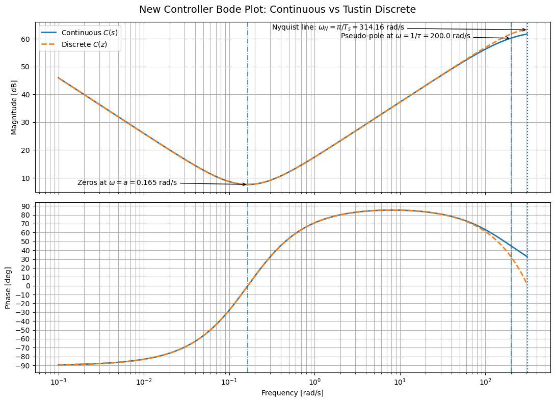
# ============================================================
# 9) PLOT: FILTER BODE, CONTINUOUS VS DISCRETE
# ============================================================
filter_breaks = [
(10.0, r'Filter pole at $\omega=10$ rad/s')
]
bode_compare_plot(
f_lp, fz,
title='Low-Pass Filter Bode Plot: Continuous vs Tustin Discrete',
label_c=r'Continuous $f(s)$',
label_d=r'Discrete $f(z)$',
annotate_breaks=filter_breaks,
show_nyquist=True
)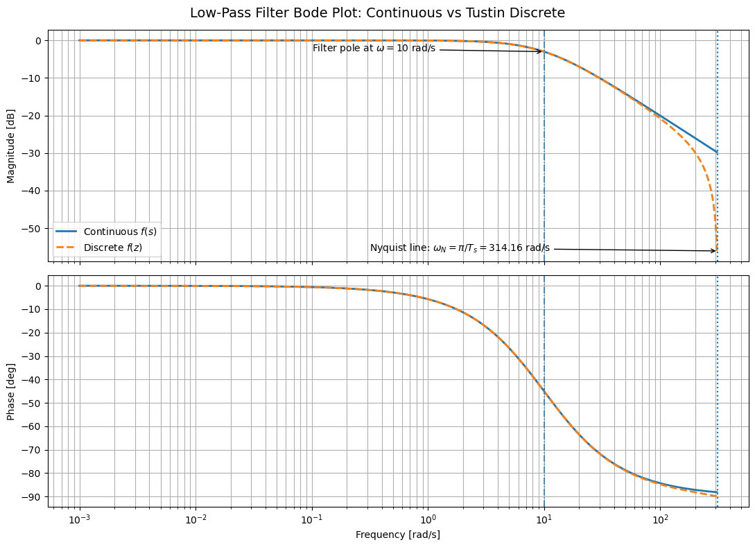
# ============================================================
# 6) HELPER FUNCTIONS
# ============================================================
def bode_data(sys, omega):
mag, phase, omega = ct.frequency_response(sys, omega)
mag = np.squeeze(mag)
phase = np.squeeze(phase)
mag_db = 20.0 * np.log10(mag)
phase_deg = np.degrees(np.unwrap(phase))
return omega, mag_db, phase_deg
def interp_logx(x, xp, fp):
return np.interp(np.log10(x), np.log10(xp), fp)
def bode_compare_plot(sys_c, sys_d, title, label_c, label_d,
annotate_breaks=None, show_nyquist=True,
show_pm=False, pm_value=None, pm_freq=None,
show_bw=False, bw_value=None):
wc, magc_db, phasec_deg = bode_data(sys_c, omega)
wd, magd_db, phased_deg = bode_data(sys_d, omega)
fig, ax = plt.subplots(2, 1, figsize=(11, 8), sharex=True)
fig.suptitle(title, fontsize=14)
# Magnitude
ax[0].semilogx(wc, magc_db, linewidth=2, label=label_c)
ax[0].semilogx(wd, magd_db, '--', linewidth=2, label=label_d)
ax[0].set_ylabel('Magnitude [dB]')
ax[0].grid(True, which='both')
ax[0].legend()
# Phase
ax[1].semilogx(wc, phasec_deg, linewidth=2, label=label_c)
ax[1].semilogx(wd, phased_deg, '--', linewidth=2, label=label_d)
ax[1].set_xlabel('Frequency [rad/s]')
ax[1].set_ylabel('Phase [deg]')
ax[1].grid(True, which='both')
# Denser phase ticks
phase_min = min(np.min(phasec_deg), np.min(phased_deg))
phase_max = max(np.max(phasec_deg), np.max(phased_deg))
yt_lo = 10 * np.floor(phase_min / 10)
yt_hi = 10 * np.ceil(phase_max / 10)
ax[1].set_yticks(np.arange(yt_lo, yt_hi + 10, 10))
if show_nyquist:
for axes in ax:
axes.axvline(w_nyq, linestyle=':', linewidth=1.6)
ax[0].annotate(
rf'Nyquist line: $\omega_N=\pi/T_s={w_nyq:.2f}$ rad/s',
xy=(w_nyq, interp_logx(0.98 * w_nyq, wd, magd_db)),
xytext=(w_nyq / 1000, interp_logx(0.98 * w_nyq, wd, magd_db) - 0),
arrowprops=dict(arrowstyle='->')
)
if annotate_breaks:
for wb, text in annotate_breaks:
for axes in ax:
axes.axvline(wb, linestyle='-.', linewidth=1.1)
ax[0].annotate(
text,
xy=(wb, interp_logx(wb, wc, magc_db)),
xytext=(wb * 1, interp_logx(wb, wc, magc_db) + 20),
arrowprops=dict(arrowstyle='->')
)
if show_pm and pm_value is not None and pm_freq is not None and np.isfinite(pm_freq) and pm_freq > 0:
for axes in ax:
axes.axvline(pm_freq, linestyle='--', linewidth=1.2)
ax[0].axhline(0, linestyle='--', linewidth=1.0)
ax[1].axhline(-180, linestyle='--', linewidth=1.0)
phase_at_pm = interp_logx(pm_freq, wc, phasec_deg)
ax[1].annotate(
rf'PM $\approx {pm_value:.2f}^\circ$ at $\omega={pm_freq:.3f}$ rad/s',
xy=(pm_freq, phase_at_pm),
xytext=(pm_freq * 1.6, phase_at_pm + 20),
arrowprops=dict(arrowstyle='->')
)
if show_bw and bw_value is not None and np.isfinite(bw_value) and bw_value > 0:
for axes in ax:
axes.axvline(bw_value, linestyle='--', linewidth=1.2)
ax[0].annotate(
rf'Bandwidth $\approx {bw_value:.3f}$ rad/s',
xy=(bw_value, interp_logx(bw_value, wc, magc_db)),
xytext=(bw_value * 1.5, interp_logx(bw_value, wc, magc_db) - 10),
arrowprops=dict(arrowstyle='->')
)
plt.tight_layout()
plt.show()# ============================================================
# 10) PLOT: PLANT BODE, CONTINUOUS VS DISCRETE
# ============================================================
plant_breaks = [
(0.02397, r'Plant pole at $\omega=0.02397$ rad/s')
]
bode_compare_plot(
P, Pz,
title='Plant Bode Plot: Continuous vs Tustin Discrete',
label_c=r'Continuous $P(s)$',
label_d=r'Discrete $P(z)$',
annotate_breaks=plant_breaks,
show_nyquist=True
)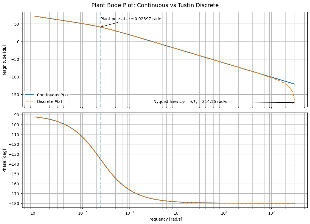
# ============================================================
# 11) CLOSED-LOOP BODE PLOT
# Continuous closed-loop transfer function
# ============================================================
omega_T, magT_db, phaseT_deg = bode_data(T, omega)
fig, ax = plt.subplots(2, 1, figsize=(11, 8), sharex=True)
fig.suptitle('Closed-Loop Bode Plot: T(s) = L(s)/(1+L(s))', fontsize=14)
ax[0].semilogx(omega_T, magT_db, linewidth=2, label=r'Closed-loop $T(s)$')
ax[0].axhline(-3, linestyle='--', linewidth=1.0)
ax[0].set_ylabel('Magnitude [dB]')
ax[0].grid(True, which='both')
ax[0].legend()
ax[1].semilogx(omega_T, phaseT_deg, linewidth=2, label=r'Closed-loop $T(s)$')
ax[1].set_xlabel('Frequency [rad/s]')
ax[1].set_ylabel('Phase [deg]')
ax[1].grid(True, which='both')
# Denser phase ticks
yt_lo = 10 * np.floor(np.min(phaseT_deg) / 10)
yt_hi = 10 * np.ceil(np.max(phaseT_deg) / 10)
ax[1].set_yticks(np.arange(yt_lo, yt_hi + 10, 10))
# Bandwidth annotation
if np.isfinite(bw_closed) and bw_closed > 0:
for axes in ax:
axes.axvline(bw_closed, linestyle='--', linewidth=1.2)
ax[0].annotate(
rf'Closed-loop bandwidth $\approx {bw_closed:.3f}$ rad/s',
xy=(bw_closed, interp_logx(bw_closed, omega_T, magT_db)),
xytext=(bw_closed * 3.5, interp_logx(bw_closed, omega_T, magT_db) - 10),
arrowprops=dict(arrowstyle='->')
)
# Phase margin note on closed-loop figure for reference
if np.isfinite(wp) and wp > 0:
ax[1].annotate(
rf'Open-loop PM $\approx {pm:.2f}^\circ$ at $\omega={wp:.3f}$ rad/s',
xy=(wp, interp_logx(wp, omega_T, phaseT_deg)),
xytext=(wp * 1.5, interp_logx(wp, omega_T, phaseT_deg) + 25),
arrowprops=dict(arrowstyle='->')
)
plt.tight_layout()
plt.show()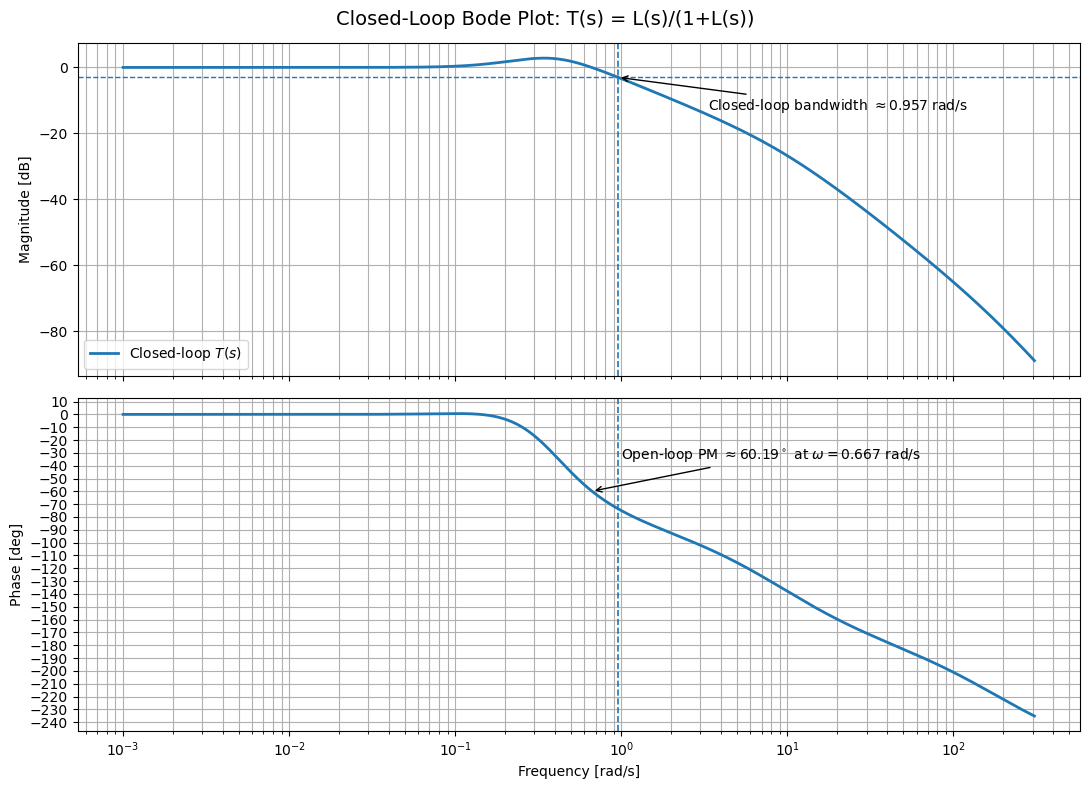
# ============================================================
# 12) CLOSED-LOOP STEP RESPONSE
# ============================================================
t = np.linspace(0, 60, 6000)
t_step, y_step = ct.step_response(T, T=t)
info = ct.step_info(T)
plt.figure(figsize=(11, 4.8))
plt.plot(t_step, y_step, linewidth=2, label='Closed-loop step response')
plt.axhline(1.0, linestyle='--', linewidth=1.0, label='Reference')
peak_idx = np.argmax(y_step)
peak_t = t_step[peak_idx]
peak_y = y_step[peak_idx]
plt.plot(peak_t, peak_y, 'o')
plt.annotate(
f'Peak = {peak_y:.4f}\n'
rf'Ts $\approx$ {info["SettlingTime"]:.3f} s\n'
rf'OS $\approx$ {info["Overshoot"]:.2f}%',
xy=(peak_t, peak_y),
xytext=(peak_t + 4, peak_y - 0.1),
arrowprops=dict(arrowstyle='->')
)
if np.isfinite(info["RiseTime"]):
plt.annotate(
rf'Rise time $\approx$ {info["RiseTime"]:.3f} s',
xy=(info["RiseTime"], np.interp(info["RiseTime"], t_step, y_step)),
xytext=(info["RiseTime"] + 5, 0.6),
arrowprops=dict(arrowstyle='->')
)
plt.title('Closed-Loop Step Response')
plt.xlabel('Time [s]')
plt.ylabel('Output')
plt.grid(True)
plt.legend()
plt.tight_layout()
plt.show()