Mark Khusid
import pandas as pd
import numpy as np

from mpl_toolkits.mplot3d import Axes3D
import matplotlib.pyplot as plt
import seaborn as sns

import pickle

from scipy.integrate import simpson
from scipy.ndimage import uniform_filter1d
from scipy.signal import find_peaks

from sklearn.impute import KNNImputer

from sklearn.svm import SVC

from sklearn.decomposition import PCA

from sklearn.model_selection import train_test_split
from sklearn.model_selection import cross_val_score

from sklearn.preprocessing import StandardScaler

from sklearn.metrics import confusion_matrix
from sklearn.metrics import accuracy_score, recall_score, precision_score, f1_score
Load the datasets
insulin_data_1 = pd.read_csv('InsulinData.csv', low_memory=False)
insulin_data_2 = pd.read_csv('Insulin_patient2.csv', low_memory=False)
cgm_data_1 = pd.read_csv('CGMData.csv', low_memory=False)
cgm_data_2 = pd.read_csv('CGM_patient2.csv', low_memory=False)
View Dataframes
#insulin_data_1#cgm_data_1#insulin_data_2#cgm_data_2EDA on dataframes
#insulin_data_1.info()#cgm_data_1.info()#insulin_data_2.info()#cgm_data_2.info()Convert ‘Date’ and ‘Time’ columns to datetime format in both datasets for easier manipulation
def preprocess_date(date_string):
    date_string = date_string.strip()
    if len(date_string.split()) == 1:
        return date_string
    elif len(date_string.split()) == 2:
        return date_string.split()[0]
insulin_data_1['Date'] = insulin_data_1['Date'].apply(preprocess_date)
insulin_data_2['Date'] = insulin_data_2['Date'].apply(preprocess_date)insulin_data_1['datetime'] = pd.to_datetime(insulin_data_1['Date'] + ' ' + insulin_data_1['Time'])
insulin_data_2['datetime'] = pd.to_datetime(insulin_data_2['Date'] + ' ' + insulin_data_2['Time'])
cgm_data_1['datetime'] = pd.to_datetime(cgm_data_1['Date'] + ' ' + cgm_data_1['Time'])
cgm_data_2['datetime'] = pd.to_datetime(cgm_data_2['Date'] + ' ' + cgm_data_2['Time'])#insulin_data_1[['Date', 'Time', 'datetime']]#insulin_data_2[['Date', 'Time', 'datetime']]#cgm_data_1[['Date', 'Time', 'datetime']]#cgm_data_2[['Date', 'Time', 'datetime']]Search for non-zero BWZ Carb Input Data
# This datetime series contains the start of all non NaN and  positive carb input
# data from the column BWZ Carb Input (grams)
meal_times_1 = \
    insulin_data_1[~insulin_data_1['BWZ Carb Input (grams)'].isna() & \
    (insulin_data_1['BWZ Carb Input (grams)'] > 0)]['datetime']
meal_times_1
48 2018-02-12 09:15:45
129 2018-02-12 02:30:55
188 2018-02-11 20:33:18
207 2018-02-11 18:14:37
222 2018-02-11 16:27:04
...
41265 2017-07-26 11:24:52
41274 2017-07-26 09:27:16
41347 2017-07-25 18:31:40
41393 2017-07-25 10:39:46
41401 2017-07-25 10:21:19
Name: datetime, Length: 747, dtype: datetime64[ns]# This datetime series contains the start of all non NaN and positive carb input
# data from the column BWZ Carb Input (grams)
meal_times_2 = \
insulin_data_2[~insulin_data_2['BWZ Carb Input (grams)'].isna() & \
(insulin_data_2['BWZ Carb Input (grams)'] > 0)]['datetime']
#meal_times_2Extract Meal Data
Obtain CGM Data based on Length of After-Meal Window
# Initialize meal data list
meal_data_1 = []

# Loop through each meal start time
for meal_time in meal_times_1:
    # A meal windows is 2 hours long
    meal_window = insulin_data_1[(insulin_data_1['datetime'] > meal_time) &
                               (insulin_data_1['datetime'] <= (meal_time + pd.Timedelta(hours=2)))]
    #print(meal_window)

    # If that meal window is empty, get corresponding CGM_
    # data that starts at tm-30 and ends at tm+2hrs
    if meal_window.empty:
        # Step 4 condition (a): No meal between tm and tm+2hrs, use this stretch as meal data
        meal_cgm_data_1 = cgm_data_1[(cgm_data_1['datetime'] >= (meal_time - pd.Timedelta(minutes=30))) &
                                 (cgm_data_1['datetime'] <= (meal_time + pd.Timedelta(hours=2)))]
    else:
        # Step 4 check for condition (b) or (c)
        next_meal_time = meal_window.iloc[0]['datetime']
        if next_meal_time < (meal_time + pd.Timedelta(hours=2)):
            # condition (b): There is a meal at tp between tm and tm+2hrs, use tp data
            meal_time = next_meal_time
            meal_cgm_data_1 = cgm_data_1[(cgm_data_1['datetime'] >= (meal_time - pd.Timedelta(minutes=30))) &
                                     (cgm_data_1['datetime'] <= (meal_time + pd.Timedelta(hours=2)))]
        # Condition (c): There is a meal exactly at tm+2hrs, use tm+1hr 30min to tm+4hrs
        elif next_meal_time == (meal_time + pd.Timedelta(hours=2)):
            meal_cgm_data_1 = cgm_data_1[(cgm_data_1['datetime'] >= (meal_time + pd.Timedelta(hours=1, minutes=30))) &
                                     (cgm_data_1['datetime'] <= (meal_time + pd.Timedelta(hours=4)))]

    # Check if the extracted data has the correct number of points (30 for meal data)
    if len(meal_cgm_data_1) == 30:
        #print(f"Meal Time Data {meal_time} has {len(meal_cgm_data)} number of points.")
        meal_data_1.append(meal_cgm_data_1['Sensor Glucose (mg/dL)'].values)
# Initialize meal data list
meal_data_2 = []
# Loop through each meal start time
for meal_time in meal_times_2:
# A meal windows is 2 hours long
meal_window = insulin_data_2[(insulin_data_2['datetime'] > meal_time) &
(insulin_data_2['datetime'] <= (meal_time + pd.Timedelta(hours=2)))]
#print(meal_window)
# If that meal window is empty, get corresponding CGM_
# data that starts at tm-30 and ends at tm+2hrs
if meal_window.empty:
# Step 4 condition (a): No meal between tm and tm+2hrs, use this stretch as meal data
meal_cgm_data_2 = cgm_data_2[(cgm_data_2['datetime'] >= (meal_time - pd.Timedelta(minutes=30))) &
(cgm_data_2['datetime'] <= (meal_time + pd.Timedelta(hours=2)))]
else:
# Step 4 check for condition (b) or (c)
next_meal_time = meal_window.iloc[0]['datetime']
if next_meal_time < (meal_time + pd.Timedelta(hours=2)):
# condition (b): There is a meal at tp between tm and tm+2hrs, use tp data
meal_time = next_meal_time
meal_cgm_data_2 = cgm_data_2[(cgm_data_2['datetime'] >= (meal_time - pd.Timedelta(minutes=30))) &
(cgm_data_2['datetime'] <= (meal_time + pd.Timedelta(hours=2)))]
# Condition (c): There is a meal exactly at tm+2hrs, use tm+1hr 30min to tm+4hrs
elif next_meal_time == (meal_time + pd.Timedelta(hours=2)):
meal_cgm_data_2 = cgm_data_2[(cgm_data_2['datetime'] >= (meal_time + pd.Timedelta(hours=1, minutes=30))) &
(cgm_data_2['datetime'] <= (meal_time + pd.Timedelta(hours=4)))]
# Check if the extracted data has the correct number of points (30 for meal data)
if len(meal_cgm_data_2) == 30:
#print(f"Meal Time Data {meal_time} has {len(meal_cgm_data)} number of points.")
meal_data_2.append(meal_cgm_data_2['Sensor Glucose (mg/dL)'].values)Get Length of Meal Data CGM Values
len(meal_data_1)715len(meal_data_2)372meal_data_1[0:5][array([ nan, nan, 124., 126., 127., 128., 130., 137., 140., nan, 150.,
140., 131., 130., 134., 148., nan, 159., 157., 140., 146., 148.,
151., 150., 162., 174., 180., 178., 184., 185.]),
array([121., 120., 115., 110., 106., 103., 103., 101., nan, 131., 109.,
82., 74., 66., 73., 82., 87., 90., 83., 73., 49., 58.,
69., 79., nan, 93., 92., 86., 84., 80.]),
array([287., 288., 289., 279., 260., 262., 259., 250., 245., 250., 247.,
243., 227., 213., 205., 182., 175., 170., 166., 164., 165., 158.,
153., 161., 177., 194., 200., 201., 189., 162.]),
array([189., 162., 166., 173., 176., 169., 167., 166., 168., 180., 182.,
178., 171., 160., 145., 138., 132., 120., 127., 129., 132., 123.,
104., 100., 107., 106., 123., 128., 137., 147.]),
array([107., 106., 123., 128., 137., 147., 145., 142., nan, nan, nan,
nan, nan, nan, nan, nan, nan, nan, nan, nan, nan, nan,
nan, nan, nan, nan, nan, nan, nan, nan])]#meal_data_2[0:5]Create Meal Data Matrix
meal_data_matrix_1 = np.array(meal_data_1)
meal_data_matrix_1
array([[ nan, nan, 124., ..., 178., 184., 185.],
[121., 120., 115., ..., 86., 84., 80.],
[287., 288., 289., ..., 201., 189., 162.],
...,
[274., 278., 283., ..., 268., 281., 292.],
[223., 222., 222., ..., 324., 326., 328.],
[ 82., 85., 92., ..., 164., 163., 155.]])meal_data_matrix_1.shape(715, 30)meal_data_matrix_2 = np.array(meal_data_2)
meal_data_matrix_2array([[390., 391., 389., ..., 165., 139., 133.],
[116., 113., 110., ..., 248., 233., 222.],
[130., 129., 126., ..., 153., 147., 147.],
...,
[174., 181., 191., ..., 126., 129., 128.],
[174., 181., 191., ..., 126., 129., 128.],
[102., 94., 92., ..., 169., 180., 186.]])meal_data_matrix_2.shape(372, 30)Visualize Meal Data Matrix 1
Heatmap of Meal Data Matrix 1
# Create the heatmap
sampled_meal_data_matrix_1 = meal_data_matrix_1[np.random.choice(meal_data_matrix_1.shape[0], 200, replace=False)]
plt.figure(figsize=(30, 30))
sns.heatmap(sampled_meal_data_matrix_1, cmap='YlGnBu', linewidths=0.5, annot=False, vmin=None, vmax=None)
plt.title('Heatmap of Meal Data Matrix 1')
plt.xlabel('Time Points')
plt.ylabel('Meals (Samples)')
plt.show()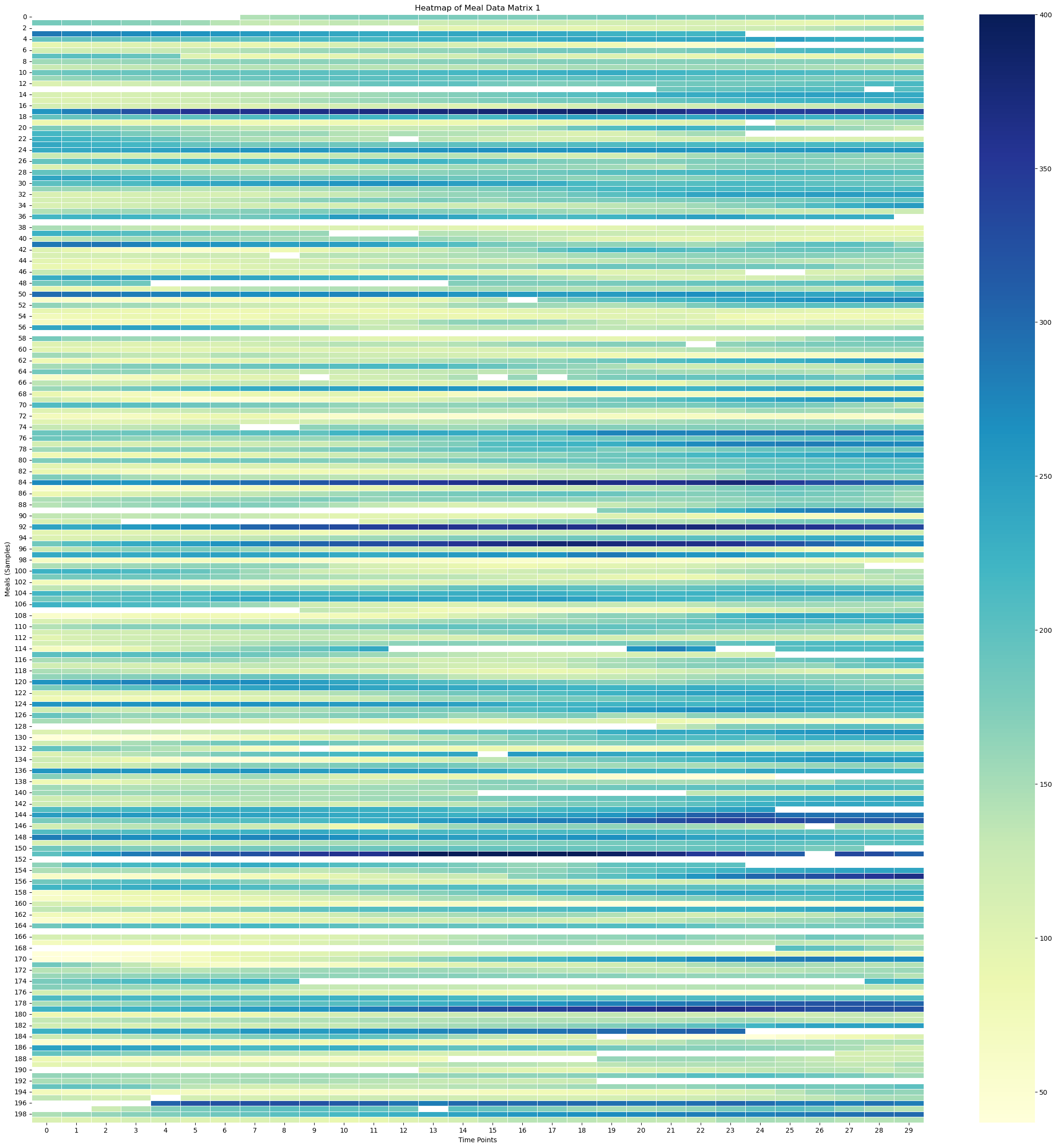
Surface Plot of Meal Data Matrix 1
# Create X, Y meshgrid
X = np.arange(meal_data_matrix_1.shape[1])
Y = np.arange(meal_data_matrix_1.shape[0])
time_points = np.linspace(-30, 120, 30)  # X-axis: from -30 minutes to +120 minutes (30 time points)
meal_numbers = np.arange(1, len(meal_data_1) + 1)
X, Y = np.meshgrid(time_points, Y)
#X, Y = np.meshgrid(time_points, meal_numbers)Xarray([[-30. , -24.82758621, -19.65517241, ..., 109.65517241,
114.82758621, 120. ],
[-30. , -24.82758621, -19.65517241, ..., 109.65517241,
114.82758621, 120. ],
[-30. , -24.82758621, -19.65517241, ..., 109.65517241,
114.82758621, 120. ],
...,
[-30. , -24.82758621, -19.65517241, ..., 109.65517241,
114.82758621, 120. ],
[-30. , -24.82758621, -19.65517241, ..., 109.65517241,
114.82758621, 120. ],
[-30. , -24.82758621, -19.65517241, ..., 109.65517241,
114.82758621, 120. ]])X.shape(715, 30)Yarray([[ 0, 0, 0, ..., 0, 0, 0],
[ 1, 1, 1, ..., 1, 1, 1],
[ 2, 2, 2, ..., 2, 2, 2],
...,
[712, 712, 712, ..., 712, 712, 712],
[713, 713, 713, ..., 713, 713, 713],
[714, 714, 714, ..., 714, 714, 714]])# Fill NaNs using forward fill, then backward fill
meal_data_matrix_1_df = pd.DataFrame(meal_data_matrix_1)
meal_data_matrix_1_filled = meal_data_matrix_1_df.ffill().bfill().values# Apply a moving average smoothing to each row
window_size = 5 # Choose a window size for smoothing
smoothed_meal_data_matrix_1 = np.array([uniform_filter1d(row, size=window_size) for row in meal_data_matrix_1_filled])# Create the plot
fig = plt.figure(figsize=(10, 8))
ax = fig.add_subplot(111, projection='3d')
stride = 100
# Plot the surface
surface_plot = ax.plot_surface(X[::stride], Y[::stride], smoothed_meal_data_matrix_1[::stride], cmap='viridis', edgecolor='none')
ax.set_title('3D Surface Plot of Smoothed Averaged Meal Glucose Levels', y=0.985)
ax.set_xlabel('Time Relative to Start of Meal [minutes]', labelpad=10)
ax.set_ylabel('Meal Samples', labelpad=10)
#ax.set_zlabel('Glucose Level (mg/dL)', labelpad=30)
#ax.set_xticks(np.linspace(-30, 120, 7))
# Adjust axis limits to create a zoom-out effect
#ax.set_xlim(-30, 120)
ax.set_ylim(0, 800)
ax.set_zlim(0, 300)
fig.colorbar(surface_plot, ax=ax, shrink=0.5, aspect=10, label='Glucose Level (mg/dL)')
#plt.tight_layout()
fig.subplots_adjust(left=0.01, right=1, top=0.9, bottom=0.1)
ax.view_init(elev=25, azim=-55)
plt.show()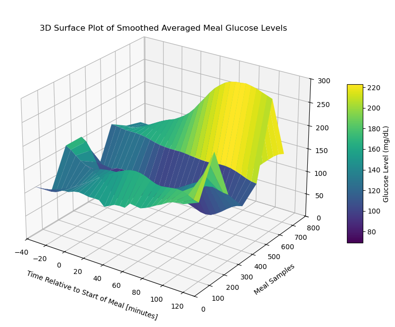
Contour Plot of Meal Data Matrix 1
# Create the contour plot
plt.figure(figsize=(15, 10))
plt.contourf(X, Y, meal_data_matrix_1_df, cmap='viridis', levels=30)
plt.colorbar(label='Glucose Level (mg/dL)')
plt.title('Contour Plot of Meal Glucose Levels')
plt.xlabel('Time Points')
plt.ylabel('Meal Samples')
plt.show()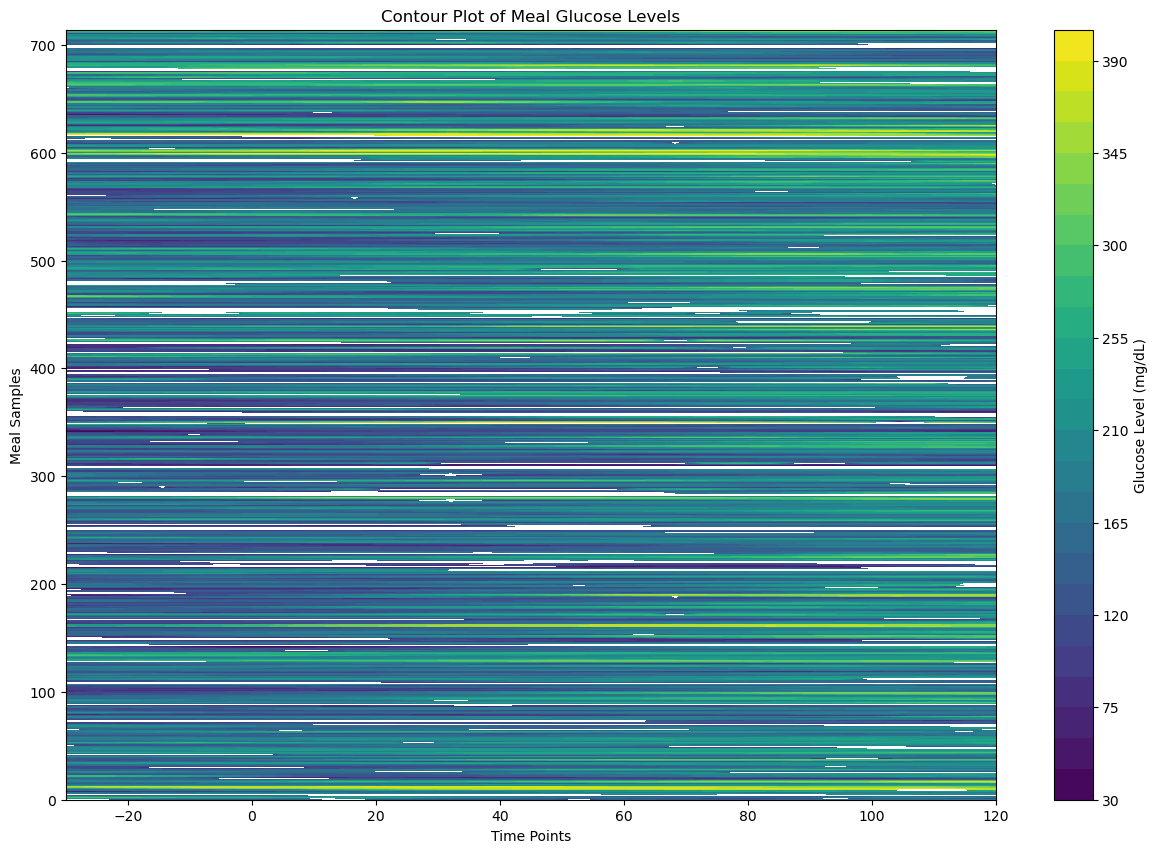
Visualize Meal Data Matrix 2
Heatmap of Meal Data Matrix 2
# Create the heatmap
sampled_meal_data_matrix_2 = meal_data_matrix_2[np.random.choice(meal_data_matrix_2.shape[0], 200, replace=False)]
plt.figure(figsize=(30, 30))
sns.heatmap(sampled_meal_data_matrix_2, cmap='YlGnBu', linewidths=0.5, annot=False, vmin=None, vmax=None)
plt.title('Heatmap of Meal Data Matrix 2')
plt.xlabel('Time Points')
plt.ylabel('Meals (Samples)')
plt.show()
Surface Plot of Meal Data Matrix 2
# Create X, Y meshgrid
X = np.arange(meal_data_matrix_2.shape[1])
Y = np.arange(meal_data_matrix_2.shape[0])
time_points = np.linspace(-30, 120, 30)  # X-axis: from -30 minutes to +120 minutes (30 time points)
meal_numbers = np.arange(1, len(meal_data_2) + 1)
X, Y = np.meshgrid(time_points, Y)
#X, Y = np.meshgrid(time_points, meal_numbers)Xarray([[-30. , -24.82758621, -19.65517241, ..., 109.65517241,
114.82758621, 120. ],
[-30. , -24.82758621, -19.65517241, ..., 109.65517241,
114.82758621, 120. ],
[-30. , -24.82758621, -19.65517241, ..., 109.65517241,
114.82758621, 120. ],
...,
[-30. , -24.82758621, -19.65517241, ..., 109.65517241,
114.82758621, 120. ],
[-30. , -24.82758621, -19.65517241, ..., 109.65517241,
114.82758621, 120. ],
[-30. , -24.82758621, -19.65517241, ..., 109.65517241,
114.82758621, 120. ]])X.shape(372, 30)Yarray([[ 0, 0, 0, ..., 0, 0, 0],
[ 1, 1, 1, ..., 1, 1, 1],
[ 2, 2, 2, ..., 2, 2, 2],
...,
[369, 369, 369, ..., 369, 369, 369],
[370, 370, 370, ..., 370, 370, 370],
[371, 371, 371, ..., 371, 371, 371]])# Fill NaNs using forward fill, then backward fill
meal_data_matrix_2_df = pd.DataFrame(meal_data_matrix_2)
meal_data_matrix_2_filled = meal_data_matrix_2_df.ffill().bfill().values# Apply a moving average smoothing to each row
window_size = 5 # Choose a window size for smoothing
smoothed_meal_data_matrix_2 = np.array([uniform_filter1d(row, size=window_size) for row in meal_data_matrix_2_filled])# Create the plot
fig = plt.figure(figsize=(10, 8))
ax = fig.add_subplot(111, projection='3d')
stride = 100
# Plot the surface
surface_plot = ax.plot_surface(X[::stride], Y[::stride], smoothed_meal_data_matrix_2[::stride], cmap='viridis', edgecolor='none')
ax.set_title('3D Surface Plot of Smoothed Averaged Meal Glucose Levels', y=0.985)
ax.set_xlabel('Time Relative to Start of Meal [minutes]', labelpad=10)
ax.set_ylabel('Meal Samples', labelpad=10)
#ax.set_zlabel('Glucose Level (mg/dL)', labelpad=30)
#ax.set_xticks(np.linspace(-30, 120, 7))
# Adjust axis limits to create a zoom-out effect
#ax.set_xlim(-30, 120)
#ax.set_ylim(0, 800)
ax.set_zlim(0, 400)
fig.colorbar(surface_plot, ax=ax, shrink=0.5, aspect=10, label='Glucose Level (mg/dL)')
#plt.tight_layout()
fig.subplots_adjust(left=0.01, right=1, top=0.9, bottom=0.1)
ax.view_init(elev=25, azim=-55)
plt.show()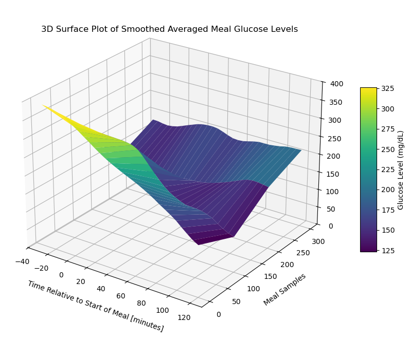
Contour Plot of Meal Data Matrix 2
# Create the contour plot
plt.figure(figsize=(15, 10))
plt.contourf(X, Y, meal_data_matrix_2_df, cmap='viridis', levels=30)
plt.colorbar(label='Glucose Level (mg/dL)')
plt.title('Contour Plot of Meal Glucose Levels')
plt.xlabel('Time Points')
plt.ylabel('Meal Samples')
plt.show()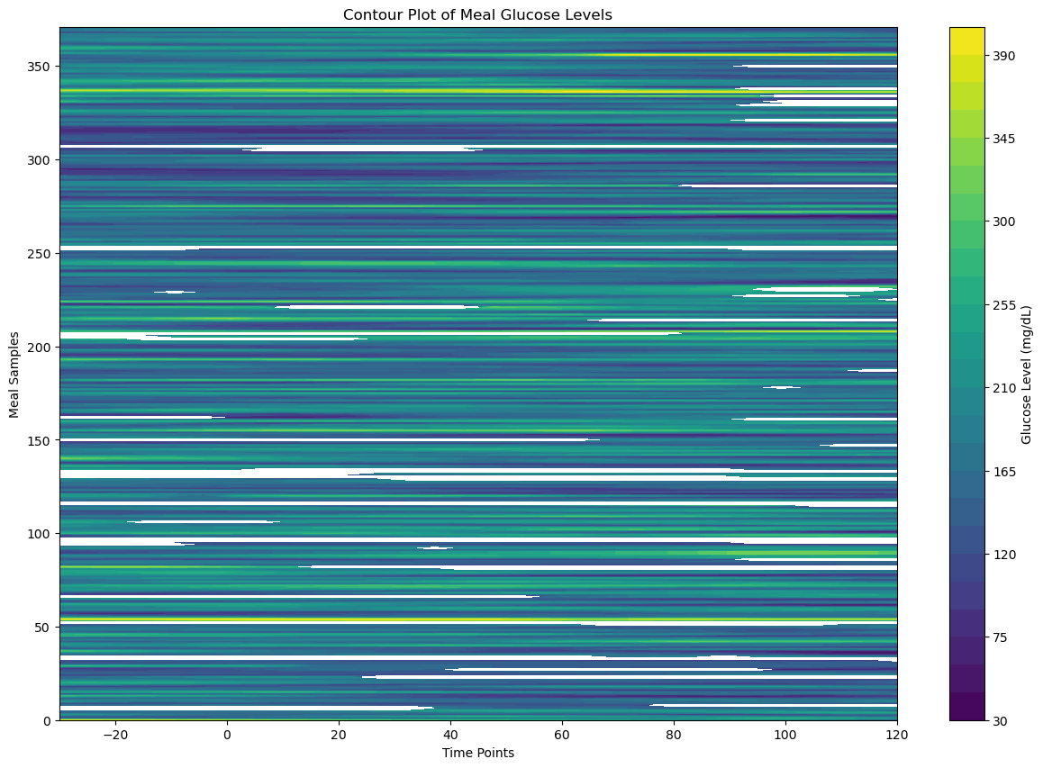
Extract No - Meal Data
# Initialize meal data list
no_meal_data_1 = []

# Loop through each meal start time to find valid post - absorbtive windows
for meal_time in meal_times_1:
    # Define the post-absorptive period: starts from tm+2 hours
    # and lasts 2 hours (i.e to four hours)
    post_absorptive_start = meal_time + pd.Timedelta(hours=2)
    post_absorptive_end = meal_time + pd.Timedelta(hours=4)

    # Check for meals in the post-absorptive period
    post_absorptive_meals = insulin_data_1[(insulin_data_1['datetime'] >= post_absorptive_start) &
                                         (insulin_data_1['datetime'] <= post_absorptive_end)]

    # Step 2 Condition (a): If any non-zero, non-NaN meal is found in the
    # post-absorptive period, skip this stretch
    if not post_absorptive_meals.empty:
        # Check if any of the meals have a non-zero carb input
        if (post_absorptive_meals['BWZ Carb Input (grams)'] > 0).any():
            # Skip this stretch, as there is a meal found in the post-absorptive period
            continue

    # Step 2 condition (b): If meal values are 0 or NaN, ignore and consider the stretch
    # Extract the corresponding 2-hour CGM data
    no_meal_cgm_data_1 = cgm_data_1[(cgm_data_1['datetime'] >= post_absorptive_start) &
                                (cgm_data_1['datetime'] <= post_absorptive_end)]

    # Check if the extracted data has the correct number of points (24 for no meal data)
    if len(no_meal_cgm_data_1) == 24:
        no_meal_data_1.append(no_meal_cgm_data_1['Sensor Glucose (mg/dL)'].values)
# Initialize meal data list
no_meal_data_2 = []
# Loop through each meal start time to find valid post - absorbtive windows
for meal_time in meal_times_2:
# Define the post-absorptive period: starts from tm+2 hours
# and lasts 2 hours (i.e to four hours)
post_absorptive_start = meal_time + pd.Timedelta(hours=2)
post_absorptive_end = meal_time + pd.Timedelta(hours=4)
# Check for meals in the post-absorptive period
post_absorptive_meals = insulin_data_2[(insulin_data_2['datetime'] >= post_absorptive_start) &
(insulin_data_2['datetime'] <= post_absorptive_end)]
# Step 2 Condition (a): If any non-zero, non-NaN meal is found in the
# post-absorptive period, skip this stretch
if not post_absorptive_meals.empty:
# Check if any of the meals have a non-zero carb input
if (post_absorptive_meals['BWZ Carb Input (grams)'] > 0).any():
# Skip this stretch, as there is a meal found in the post-absorptive period
continue
# Step 2 condition (b): If meal values are 0 or NaN, ignore and consider the stretch
# Extract the corresponding 2-hour CGM data
no_meal_cgm_data_2 = cgm_data_2[(cgm_data_2['datetime'] >= post_absorptive_start) &
(cgm_data_2['datetime'] <= post_absorptive_end)]
# Check if the extracted data has the correct number of points (24 for no meal data)
if len(no_meal_cgm_data_2) == 24:
no_meal_data_2.append(no_meal_cgm_data_2['Sensor Glucose (mg/dL)'].values)len(no_meal_data_1)510len(no_meal_data_2)325#no_meal_data_1[0:5]#no_meal_data_2[0:5]Create No Meal Data Matrix
no_meal_data_matrix_1 = np.array(no_meal_data_1)
#no_meal_data_matrix_1
no_meal_data_matrix_2 = np.array(no_meal_data_2)
#no_meal_data_matrix_2no_meal_data_matrix_1.shape(510, 24)no_meal_data_matrix_2.shape(325, 24)Visualize No Meal Data Matrix 1
Heatmap of No Meal Data Matrix 1
# Create the heatmap
sampled_no_meal_data_matrix_1 = no_meal_data_matrix_1[np.random.choice(no_meal_data_matrix_1.shape[0], 200, replace=False)]
plt.figure(figsize=(30, 30))
sns.heatmap(sampled_no_meal_data_matrix_1, cmap='YlGnBu', linewidths=0.5, annot=False, vmin=None, vmax=None)
plt.title('Heatmap of No Meal Data Matrix 1')
plt.xlabel('Time Points')
plt.ylabel('Meals (Samples)')
plt.show()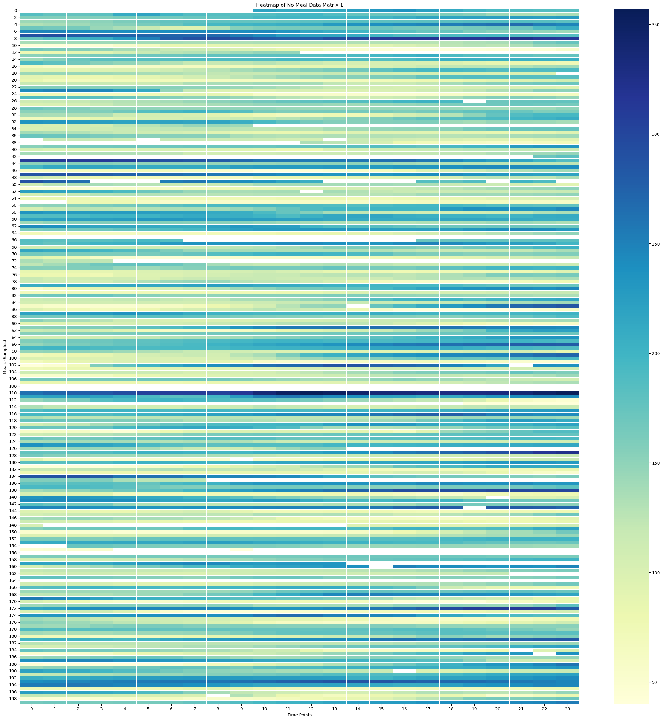
Surface Plot of No Meal Data Matrix 1
time_points = np.linspace(-30, 120, 24)
print(time_points)
print(time_points.shape)
[-30. -23.47826087 -16.95652174 -10.43478261 -3.91304348
2.60869565 9.13043478 15.65217391 22.17391304 28.69565217
35.2173913 41.73913043 48.26086957 54.7826087 61.30434783
67.82608696 74.34782609 80.86956522 87.39130435 93.91304348
100.43478261 106.95652174 113.47826087 120. ]
(24,)
# Create X, Y meshgrid
X = np.arange(no_meal_data_matrix_1.shape[1])
Y = np.arange(no_meal_data_matrix_1.shape[0])
time_points = np.linspace(-30, 120, 24)  # X-axis: from -30 minutes to +120 minutes (24 time points)
meal_numbers = np.arange(1, len(no_meal_data_1) + 1)
X, Y = np.meshgrid(time_points, Y)
#X, Y = np.meshgrid(time_points, meal_numbers)Xarray([[-30. , -23.47826087, -16.95652174, ..., 106.95652174,
113.47826087, 120. ],
[-30. , -23.47826087, -16.95652174, ..., 106.95652174,
113.47826087, 120. ],
[-30. , -23.47826087, -16.95652174, ..., 106.95652174,
113.47826087, 120. ],
...,
[-30. , -23.47826087, -16.95652174, ..., 106.95652174,
113.47826087, 120. ],
[-30. , -23.47826087, -16.95652174, ..., 106.95652174,
113.47826087, 120. ],
[-30. , -23.47826087, -16.95652174, ..., 106.95652174,
113.47826087, 120. ]])X.shape(510, 24)Yarray([[ 0, 0, 0, ..., 0, 0, 0],
[ 1, 1, 1, ..., 1, 1, 1],
[ 2, 2, 2, ..., 2, 2, 2],
...,
[507, 507, 507, ..., 507, 507, 507],
[508, 508, 508, ..., 508, 508, 508],
[509, 509, 509, ..., 509, 509, 509]])Y.shape(510, 24)# Fill NaNs using forward fill, then backward fill
no_meal_data_matrix_1_df = pd.DataFrame(no_meal_data_matrix_1)
no_meal_data_matrix_1_filled = no_meal_data_matrix_1_df.ffill().bfill().values# Apply a moving average smoothing to each row
window_size = 5 # Choose a window size for smoothing
smoothed_no_meal_data_matrix_1 = np.array([uniform_filter1d(row, size=window_size) for row in no_meal_data_matrix_1_filled])# Create the plot
fig = plt.figure(figsize=(10, 8))
ax = fig.add_subplot(111, projection='3d')
stride = 100
# Plot the surface
surface_plot = ax.plot_surface(X[::stride], Y[::stride], smoothed_no_meal_data_matrix_1[::stride], cmap='viridis', edgecolor='none')
ax.set_title('3D Surface Plot of Smoothed Averaged No Meal Glucose Levels', y=0.985)
ax.set_xlabel('Time Relative to End of Meal [minutes]', labelpad=10)
ax.set_ylabel('Meal Samples', labelpad=10)
#ax.set_zlabel('Glucose Level (mg/dL)', labelpad=30)
#ax.set_xticks(np.linspace(-30, 120, 7))
# Adjust axis limits to create a zoom-out effect
#ax.set_xlim(-30, 120)
#ax.set_ylim(0, 800)
#ax.set_zlim(0, 300)
fig.colorbar(surface_plot, ax=ax, shrink=0.5, aspect=10, label='Glucose Level (mg/dL)')
#plt.tight_layout()
fig.subplots_adjust(left=0.01, right=1, top=0.9, bottom=0.1)
ax.view_init(elev=25, azim=-55)
plt.show()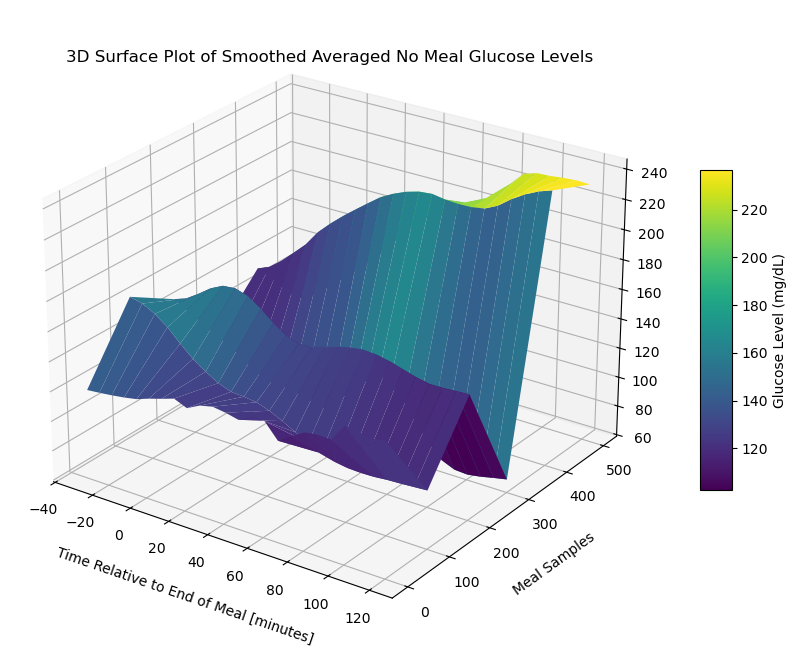
Contour Plot of No Meal Data Matrix 1
# Create the contour plot
plt.figure(figsize=(15, 10))
plt.contourf(X, Y, no_meal_data_matrix_1_df, cmap='viridis', levels=30)
plt.colorbar(label='Glucose Level (mg/dL)')
plt.title('Contour Plot of No Meal Glucose Levels')
plt.xlabel('Time Points')
plt.ylabel('Meal Samples')
plt.show()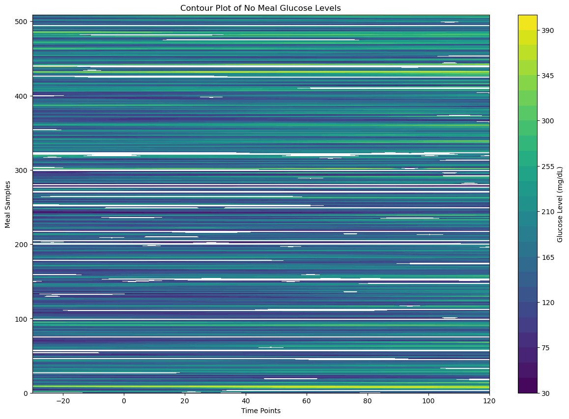
Visualize No Meal Data Matrix 2
Heatmap of No Meal Data Matrix 2
# Create the heatmap
sampled_no_meal_data_matrix_2 = no_meal_data_matrix_2[np.random.choice(no_meal_data_matrix_2.shape[0], 200, replace=False)]
plt.figure(figsize=(30, 30))
sns.heatmap(sampled_meal_data_matrix_2, cmap='YlGnBu', linewidths=0.5, annot=False, vmin=None, vmax=None)
plt.title('Heatmap of No Meal Data Matrix 1')
plt.xlabel('Time Points')
plt.ylabel('Meals (Samples)')
plt.show()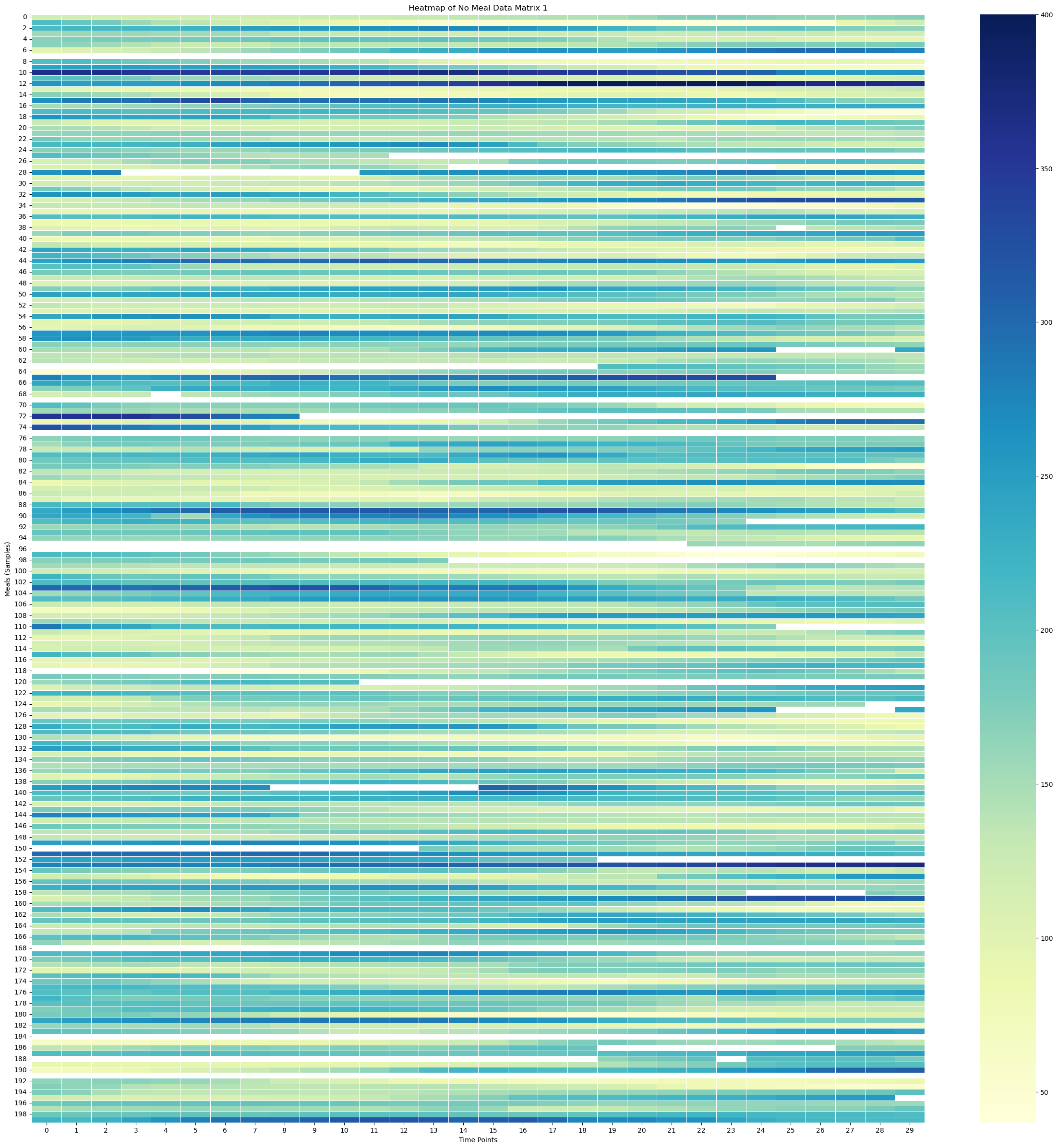
Surface Plot of No Meal Data Matrix 2
time_points = np.linspace(-30, 120, 24)
print(time_points)
print(time_points.shape)
[-30. -23.47826087 -16.95652174 -10.43478261 -3.91304348
2.60869565 9.13043478 15.65217391 22.17391304 28.69565217
35.2173913 41.73913043 48.26086957 54.7826087 61.30434783
67.82608696 74.34782609 80.86956522 87.39130435 93.91304348
100.43478261 106.95652174 113.47826087 120. ]
(24,)
# Create X, Y meshgrid
X = np.arange(no_meal_data_matrix_2.shape[1])
Y = np.arange(no_meal_data_matrix_2.shape[0])
time_points = np.linspace(-30, 120, 24)  # X-axis: from -30 minutes to +120 minutes (24 time points)
meal_numbers = np.arange(1, len(no_meal_data_2) + 1)
X, Y = np.meshgrid(time_points, Y)
#X, Y = np.meshgrid(time_points, meal_numbers)Xarray([[-30. , -23.47826087, -16.95652174, ..., 106.95652174,
113.47826087, 120. ],
[-30. , -23.47826087, -16.95652174, ..., 106.95652174,
113.47826087, 120. ],
[-30. , -23.47826087, -16.95652174, ..., 106.95652174,
113.47826087, 120. ],
...,
[-30. , -23.47826087, -16.95652174, ..., 106.95652174,
113.47826087, 120. ],
[-30. , -23.47826087, -16.95652174, ..., 106.95652174,
113.47826087, 120. ],
[-30. , -23.47826087, -16.95652174, ..., 106.95652174,
113.47826087, 120. ]])X.shape(325, 24)Yarray([[ 0, 0, 0, ..., 0, 0, 0],
[ 1, 1, 1, ..., 1, 1, 1],
[ 2, 2, 2, ..., 2, 2, 2],
...,
[322, 322, 322, ..., 322, 322, 322],
[323, 323, 323, ..., 323, 323, 323],
[324, 324, 324, ..., 324, 324, 324]])Y.shape(325, 24)# Fill NaNs using forward fill, then backward fill
no_meal_data_matrix_2_df = pd.DataFrame(no_meal_data_matrix_2)
no_meal_data_matrix_2_filled = no_meal_data_matrix_2_df.ffill().bfill().values# Apply a moving average smoothing to each row
window_size = 5 # Choose a window size for smoothing
smoothed_no_meal_data_matrix_2 = np.array([uniform_filter1d(row, size=window_size) for row in no_meal_data_matrix_2_filled])# Create the plot
fig = plt.figure(figsize=(10, 8))
ax = fig.add_subplot(111, projection='3d')
stride = 100
# Plot the surface
surface_plot = ax.plot_surface(X[::stride], Y[::stride], smoothed_no_meal_data_matrix_2[::stride], cmap='viridis', edgecolor='none')
ax.set_title('3D Surface Plot of Smoothed Averaged No Meal Glucose Levels', y=0.985)
ax.set_xlabel('Time Relative to End of Meal [minutes]', labelpad=10)
ax.set_ylabel('Meal Samples', labelpad=10)
#ax.set_zlabel('Glucose Level (mg/dL)', labelpad=30)
#ax.set_xticks(np.linspace(-30, 120, 7))
# Adjust axis limits to create a zoom-out effect
#ax.set_xlim(-30, 120)
#ax.set_ylim(0, 800)
#ax.set_zlim(0, 300)
fig.colorbar(surface_plot, ax=ax, shrink=0.5, aspect=10, label='Glucose Level (mg/dL)')
#plt.tight_layout()
fig.subplots_adjust(left=0.01, right=1, top=0.9, bottom=0.1)
ax.view_init(elev=25, azim=-55)
plt.show()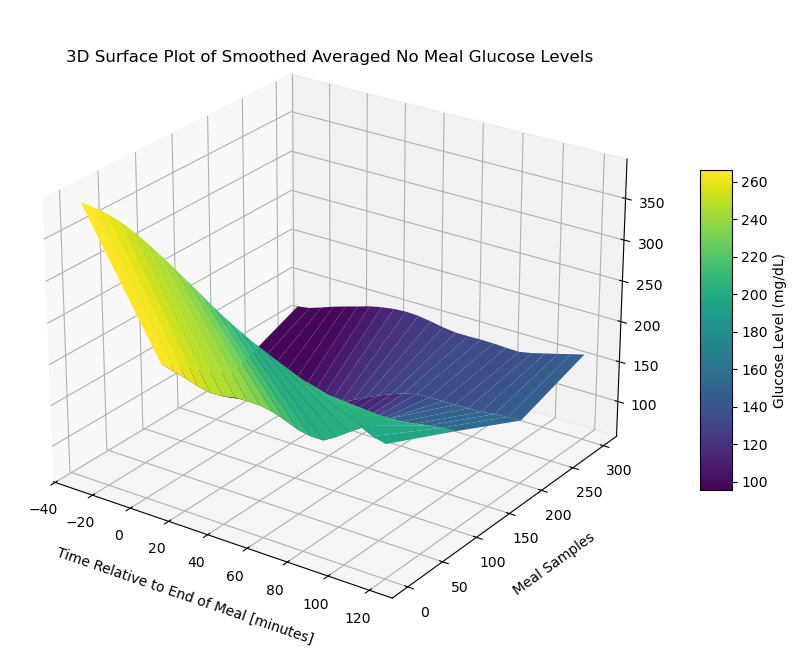
Contour Plot of No Meal Data Matrix 2
# Create the contour plot
plt.figure(figsize=(15, 10))
plt.contourf(X, Y, no_meal_data_matrix_2_df, cmap='viridis', levels=30)
plt.colorbar(label='Glucose Level (mg/dL)')
plt.title('Contour Plot of No Meal Glucose Levels')
plt.xlabel('Time Points')
plt.ylabel('Meal Samples')
plt.show()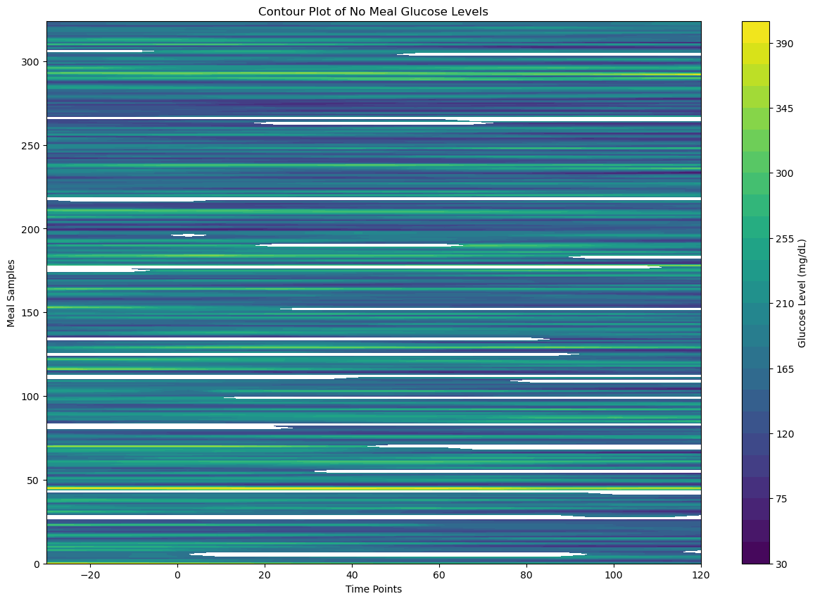
Handle Missing Data
We will use a strategy of deleting rows of data that have more than 10% of bad data. If less than 10%, we will use KNN with a nearest neighbor hyperparameter (K=7).
Define Threshold for Dumping Data
# 10%
dump_thresold = 0.1
Create KNN Imputer
knn_imputer = KNNImputer(n_neighbors=7)Parse Meal Data and Handle Missing Values
cleaned_meal_data_1 = []
for row in meal_data_matrix_1:

    proportion_missing_data = np.isnan(row).mean()

    if proportion_missing_data > dump_thresold:

        # Ignore this row
        print(f"Ignoring row with {proportion_missing_data*100:.2f}% missing data")
        continue

    else:
        # The data is good, use it
        cleaned_meal_data_1.append(row)
Ignoring row with 13.33% missing data
Ignoring row with 73.33% missing data
Ignoring row with 66.67% missing data
Ignoring row with 13.33% missing data
Ignoring row with 30.00% missing data
Ignoring row with 16.67% missing data
Ignoring row with 23.33% missing data
Ignoring row with 16.67% missing data
Ignoring row with 26.67% missing data
Ignoring row with 30.00% missing data
Ignoring row with 20.00% missing data
Ignoring row with 73.33% missing data
Ignoring row with 63.33% missing data
Ignoring row with 100.00% missing data
Ignoring row with 100.00% missing data
Ignoring row with 33.33% missing data
Ignoring row with 16.67% missing data
Ignoring row with 16.67% missing data
Ignoring row with 100.00% missing data
Ignoring row with 60.00% missing data
Ignoring row with 16.67% missing data
Ignoring row with 36.67% missing data
Ignoring row with 43.33% missing data
Ignoring row with 13.33% missing data
Ignoring row with 13.33% missing data
Ignoring row with 60.00% missing data
Ignoring row with 16.67% missing data
Ignoring row with 53.33% missing data
Ignoring row with 33.33% missing data
Ignoring row with 13.33% missing data
Ignoring row with 20.00% missing data
Ignoring row with 83.33% missing data
Ignoring row with 86.67% missing data
Ignoring row with 70.00% missing data
Ignoring row with 16.67% missing data
Ignoring row with 100.00% missing data
Ignoring row with 100.00% missing data
Ignoring row with 16.67% missing data
Ignoring row with 43.33% missing data
Ignoring row with 100.00% missing data
Ignoring row with 100.00% missing data
Ignoring row with 63.33% missing data
Ignoring row with 63.33% missing data
Ignoring row with 26.67% missing data
Ignoring row with 60.00% missing data
Ignoring row with 100.00% missing data
Ignoring row with 100.00% missing data
Ignoring row with 33.33% missing data
Ignoring row with 96.67% missing data
Ignoring row with 100.00% missing data
Ignoring row with 100.00% missing data
Ignoring row with 100.00% missing data
Ignoring row with 20.00% missing data
Ignoring row with 80.00% missing data
Ignoring row with 43.33% missing data
Ignoring row with 100.00% missing data
Ignoring row with 16.67% missing data
Ignoring row with 100.00% missing data
Ignoring row with 70.00% missing data
Ignoring row with 16.67% missing data
Ignoring row with 83.33% missing data
Ignoring row with 83.33% missing data
Ignoring row with 30.00% missing data
Ignoring row with 16.67% missing data
Ignoring row with 100.00% missing data
Ignoring row with 20.00% missing data
Ignoring row with 30.00% missing data
Ignoring row with 20.00% missing data
Ignoring row with 76.67% missing data
Ignoring row with 73.33% missing data
Ignoring row with 70.00% missing data
Ignoring row with 36.67% missing data
Ignoring row with 20.00% missing data
Ignoring row with 16.67% missing data
Ignoring row with 36.67% missing data
Ignoring row with 16.67% missing data
Ignoring row with 63.33% missing data
Ignoring row with 13.33% missing data
Ignoring row with 20.00% missing data
Ignoring row with 26.67% missing data
Ignoring row with 90.00% missing data
Ignoring row with 23.33% missing data
Ignoring row with 33.33% missing data
Ignoring row with 100.00% missing data
Ignoring row with 80.00% missing data
Ignoring row with 33.33% missing data
Ignoring row with 30.00% missing data
Ignoring row with 20.00% missing data
Ignoring row with 33.33% missing data
Ignoring row with 100.00% missing data
Ignoring row with 100.00% missing data
Ignoring row with 13.33% missing data
Ignoring row with 20.00% missing data
Ignoring row with 100.00% missing data
Ignoring row with 100.00% missing data
Ignoring row with 16.67% missing data
cleaned_meal_data_2 = []
for row in meal_data_matrix_2:

    proportion_missing_data = np.isnan(row).mean()

    if proportion_missing_data > dump_thresold:

        # Ignore this row
        print(f"Ignoring row with {proportion_missing_data*100:.2f}% missing data")
        continue

    else:
        # The data is good, use it
        cleaned_meal_data_2.append(row)
Ignoring row with 43.33% missing data
Ignoring row with 43.33% missing data
Ignoring row with 30.00% missing data
Ignoring row with 63.33% missing data
Ignoring row with 36.67% missing data
Ignoring row with 100.00% missing data
Ignoring row with 66.67% missing data
Ignoring row with 26.67% missing data
Ignoring row with 100.00% missing data
Ignoring row with 56.67% missing data
Ignoring row with 53.33% missing data
Ignoring row with 70.00% missing data
Ignoring row with 20.00% missing data
Ignoring row with 16.67% missing data
Ignoring row with 20.00% missing data
Ignoring row with 100.00% missing data
Ignoring row with 100.00% missing data
Ignoring row with 16.67% missing data
Ignoring row with 13.33% missing data
Ignoring row with 100.00% missing data
Ignoring row with 60.00% missing data
Ignoring row with 80.00% missing data
Ignoring row with 36.67% missing data
Ignoring row with 100.00% missing data
Ignoring row with 56.67% missing data
Ignoring row with 63.33% missing data
Ignoring row with 20.00% missing data
Ignoring row with 20.00% missing data
Ignoring row with 26.67% missing data
Ignoring row with 13.33% missing data
Ignoring row with 73.33% missing data
Ignoring row with 36.67% missing data
Ignoring row with 23.33% missing data
Ignoring row with 13.33% missing data
Ignoring row with 13.33% missing data
Ignoring row with 13.33% missing data
Ignoring row with 36.67% missing data
Ignoring row with 100.00% missing data
Ignoring row with 26.67% missing data
Ignoring row with 26.67% missing data
Ignoring row with 100.00% missing data
Ignoring row with 20.00% missing data
Ignoring row with 20.00% missing data
Ignoring row with 16.67% missing data
Ignoring row with 16.67% missing data
Ignoring row with 20.00% missing data
Ignoring row with 20.00% missing data
cleaned_meal_data_1[0]array([121., 120., 115., 110., 106., 103., 103., 101., nan, 131., 109.,
82., 74., 66., 73., 82., 87., 90., 83., 73., 49., 58.,
69., 79., nan, 93., 92., 86., 84., 80.])cleaned_meal_data_2[0]array([390., 391., 389., 383., 375., 368., 357., 349., 336., 326., 315.,
305., 295., 286., 279., 273., 268., 259., 252., 246., 238., 229.,
218., 206., 195., 192., 181., 165., 139., 133.])Convert Cleaned Meal Data List into a Matrix
cleaned_meal_data_matrix_1 = \
    np.array(cleaned_meal_data_1)
cleaned_meal_data_matrix_2 = \
np.array(cleaned_meal_data_2)Use KNN to Impute NaNs in Cleaned Meal Data
cleaned_imputed_meal_matrix_1 = knn_imputer.fit_transform(cleaned_meal_data_matrix_1)cleaned_imputed_meal_matrix_2 = knn_imputer.fit_transform(cleaned_meal_data_matrix_2)cleaned_imputed_meal_matrix_1[0]array([121. , 120. , 115. , 110. ,
106. , 103. , 103. , 101. ,
99.71428571, 131. , 109. , 82. ,
74. , 66. , 73. , 82. ,
87. , 90. , 83. , 73. ,
49. , 58. , 69. , 79. ,
75.85714286, 93. , 92. , 86. ,
84. , 80. ])cleaned_imputed_meal_matrix_1.shape(619, 30)cleaned_imputed_meal_matrix_2[0]array([390., 391., 389., 383., 375., 368., 357., 349., 336., 326., 315.,
305., 295., 286., 279., 273., 268., 259., 252., 246., 238., 229.,
218., 206., 195., 192., 181., 165., 139., 133.])cleaned_imputed_meal_matrix_2.shape(325, 30)Parse No Meal Data and Handle Missing Values
cleaned_no_meal_data_1 = []
for row in no_meal_data_matrix_1:

    proportion_missing_data = np.isnan(row).mean()

    if proportion_missing_data > dump_thresold:

        # Ignore this row
        print(f"Ignoring row with {proportion_missing_data*100:.2f}% missing data")
        continue

    else:
        # The data is good, use it
        cleaned_no_meal_data_1.append(row)
Ignoring row with 20.83% missing data
Ignoring row with 58.33% missing data
Ignoring row with 12.50% missing data
Ignoring row with 33.33% missing data
Ignoring row with 12.50% missing data
Ignoring row with 41.67% missing data
Ignoring row with 79.17% missing data
Ignoring row with 16.67% missing data
Ignoring row with 100.00% missing data
Ignoring row with 100.00% missing data
Ignoring row with 100.00% missing data
Ignoring row with 66.67% missing data
Ignoring row with 50.00% missing data
Ignoring row with 16.67% missing data
Ignoring row with 29.17% missing data
Ignoring row with 12.50% missing data
Ignoring row with 66.67% missing data
Ignoring row with 83.33% missing data
Ignoring row with 12.50% missing data
Ignoring row with 16.67% missing data
Ignoring row with 20.83% missing data
Ignoring row with 54.17% missing data
Ignoring row with 100.00% missing data
Ignoring row with 91.67% missing data
Ignoring row with 100.00% missing data
Ignoring row with 12.50% missing data
Ignoring row with 12.50% missing data
Ignoring row with 100.00% missing data
Ignoring row with 12.50% missing data
Ignoring row with 12.50% missing data
Ignoring row with 79.17% missing data
Ignoring row with 62.50% missing data
Ignoring row with 54.17% missing data
Ignoring row with 100.00% missing data
Ignoring row with 100.00% missing data
Ignoring row with 100.00% missing data
Ignoring row with 100.00% missing data
Ignoring row with 12.50% missing data
Ignoring row with 100.00% missing data
Ignoring row with 50.00% missing data
Ignoring row with 12.50% missing data
Ignoring row with 37.50% missing data
Ignoring row with 91.67% missing data
Ignoring row with 87.50% missing data
Ignoring row with 66.67% missing data
Ignoring row with 41.67% missing data
Ignoring row with 87.50% missing data
Ignoring row with 41.67% missing data
Ignoring row with 87.50% missing data
Ignoring row with 100.00% missing data
Ignoring row with 12.50% missing data
Ignoring row with 41.67% missing data
Ignoring row with 29.17% missing data
Ignoring row with 100.00% missing data
cleaned_no_meal_data_2 = []
for row in no_meal_data_matrix_2:

    proportion_missing_data = np.isnan(row).mean()

    if proportion_missing_data > dump_thresold:

        # Ignore this row
        print(f"Ignoring row with {proportion_missing_data*100:.2f}% missing data")
        continue

    else:
        # The data is good, use it
        cleaned_no_meal_data_2.append(row)
Ignoring row with 54.17% missing data
Ignoring row with 54.17% missing data
Ignoring row with 100.00% missing data
Ignoring row with 83.33% missing data
Ignoring row with 16.67% missing data
Ignoring row with 100.00% missing data
Ignoring row with 58.33% missing data
Ignoring row with 37.50% missing data
Ignoring row with 50.00% missing data
Ignoring row with 37.50% missing data
Ignoring row with 100.00% missing data
Ignoring row with 70.83% missing data
Ignoring row with 29.17% missing data
Ignoring row with 45.83% missing data
Ignoring row with 100.00% missing data
Ignoring row with 79.17% missing data
Ignoring row with 75.00% missing data
Ignoring row with 62.50% missing data
Ignoring row with 16.67% missing data
Ignoring row with 91.67% missing data
Ignoring row with 20.83% missing data
Ignoring row with 29.17% missing data
Ignoring row with 20.83% missing data
Ignoring row with 100.00% missing data
Ignoring row with 33.33% missing data
Ignoring row with 37.50% missing data
Ignoring row with 100.00% missing data
Ignoring row with 45.83% missing data
Ignoring row with 16.67% missing data
cleaned_no_meal_data_1[0]array([121., 120., 115., 110., 106., 103., 103., 101., nan, 131., 109.,
82., 74., 66., 73., 82., 87., 90., 83., 73., 49., 58.,
69., 79.])cleaned_no_meal_data_2[0]array([390., 391., 389., 383., 375., 368., 357., 349., 336., 326., 315.,
305., 295., 286., 279., 273., 268., 259., 252., 246., 238., 229.,
218., 206.])cleaned_no_meal_data_1[0].shape(24,)cleaned_no_meal_data_2[0].shape(24,)Convert Cleaned No Meal Data List into a Matrix
cleaned_no_meal_data_matrix_1 = \
    np.array(cleaned_no_meal_data_1)
cleaned_no_meal_data_matrix_2 = \
np.array(cleaned_no_meal_data_2)Use KNN to Impute NaNs in Cleaned No Meal Data
cleaned_imputed_no_meal_matrix_1 = knn_imputer.fit_transform(cleaned_no_meal_data_matrix_1)cleaned_imputed_no_meal_matrix_2 = knn_imputer.fit_transform(cleaned_no_meal_data_matrix_2)cleaned_imputed_no_meal_matrix_1[0]array([121. , 120. , 115. , 110. ,
106. , 103. , 103. , 101. ,
103.85714286, 131. , 109. , 82. ,
74. , 66. , 73. , 82. ,
87. , 90. , 83. , 73. ,
49. , 58. , 69. , 79. ])cleaned_imputed_no_meal_matrix_2[0]array([390., 391., 389., 383., 375., 368., 357., 349., 336., 326., 315.,
305., 295., 286., 279., 273., 268., 259., 252., 246., 238., 229.,
218., 206.])Visualize Cleaned Imputed Data
Visualize Cleaned Imputed Meal Data Matrix 1
Heatmap of Cleaned Imputed Meal Data Matrix 1
# Create the heatmap
sampled_meal_data_matrix_1 = cleaned_imputed_meal_matrix_1[np.random.choice(cleaned_imputed_meal_matrix_1.shape[0], 200, replace=False)]
plt.figure(figsize=(30, 30))
sns.heatmap(sampled_meal_data_matrix_1, cmap='YlGnBu', linewidths=0.5, annot=False, vmin=None, vmax=None)
plt.title('Heatmap of Meal Data Matrix 1', fontsize=30)
plt.xlabel('Time Points', fontsize=26)
plt.ylabel('Meals (Samples)', fontsize=26)

# Change font properties for the x and y tick labels
plt.xticks(fontsize=16)
plt.yticks(fontsize=16)

plt.show()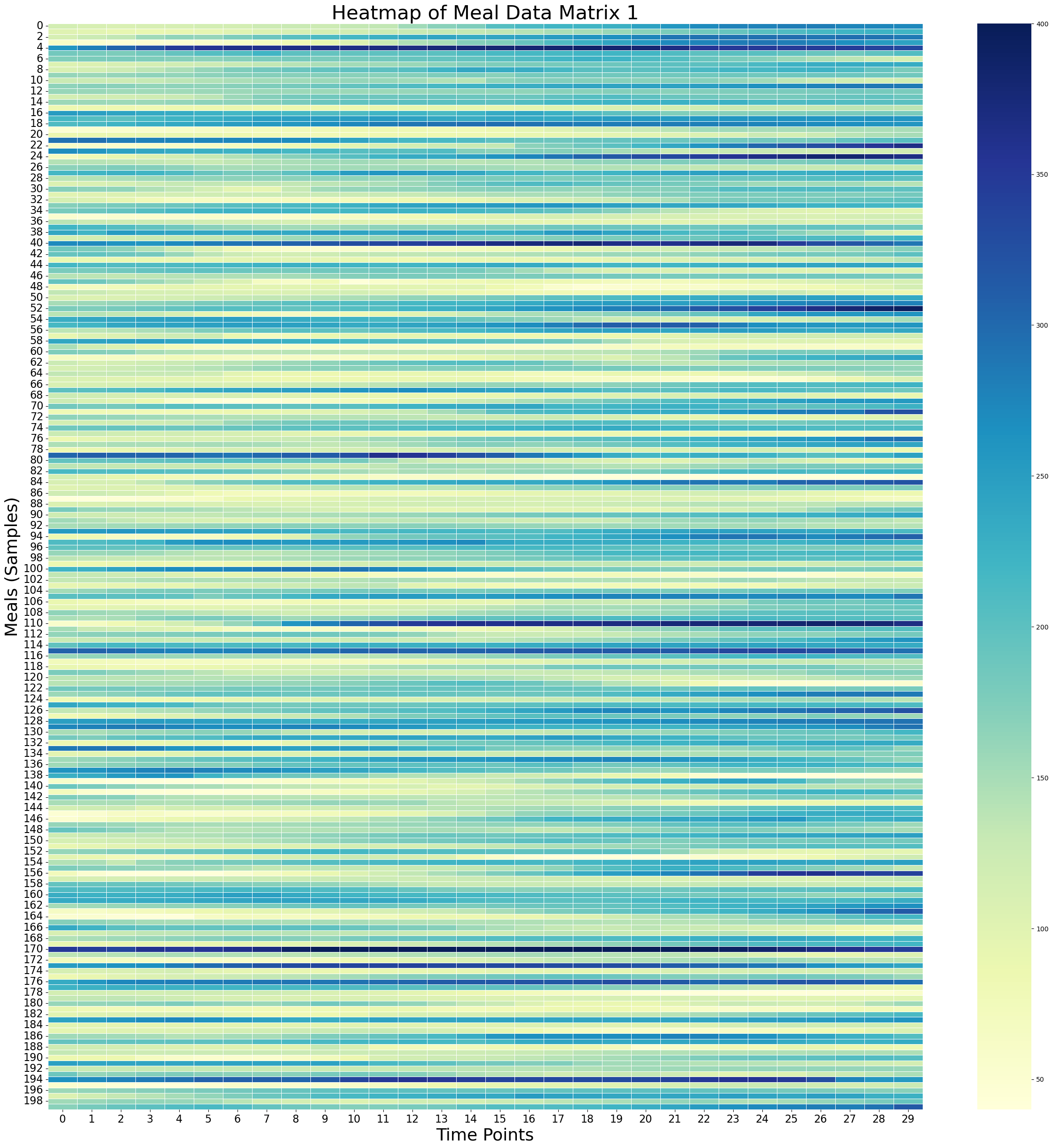
Surface Plot of Cleaned Imputed Meal Data Matrix 1
# Create X, Y meshgrid
X = np.arange(cleaned_imputed_meal_matrix_1.shape[1])
Y = np.arange(cleaned_imputed_meal_matrix_1.shape[0])
time_points = np.linspace(-30, 120, 30)  # X-axis: from -30 minutes to +120 minutes (30 time points)
meal_numbers = np.arange(1, len(meal_data_1) + 1)
X, Y = np.meshgrid(time_points, Y)
#X, Y = np.meshgrid(time_points, meal_numbers)Xarray([[-30. , -24.82758621, -19.65517241, ..., 109.65517241,
114.82758621, 120. ],
[-30. , -24.82758621, -19.65517241, ..., 109.65517241,
114.82758621, 120. ],
[-30. , -24.82758621, -19.65517241, ..., 109.65517241,
114.82758621, 120. ],
...,
[-30. , -24.82758621, -19.65517241, ..., 109.65517241,
114.82758621, 120. ],
[-30. , -24.82758621, -19.65517241, ..., 109.65517241,
114.82758621, 120. ],
[-30. , -24.82758621, -19.65517241, ..., 109.65517241,
114.82758621, 120. ]])X.shape(619, 30)Yarray([[ 0, 0, 0, ..., 0, 0, 0],
[ 1, 1, 1, ..., 1, 1, 1],
[ 2, 2, 2, ..., 2, 2, 2],
...,
[616, 616, 616, ..., 616, 616, 616],
[617, 617, 617, ..., 617, 617, 617],
[618, 618, 618, ..., 618, 618, 618]])# Fill NaNs using forward fill, then backward fill
meal_data_matrix_1_df = pd.DataFrame(cleaned_imputed_meal_matrix_1)
meal_data_matrix_1_filled = meal_data_matrix_1_df.ffill().bfill().values# Apply a moving average smoothing to each row
window_size = 3 # Choose a window size for smoothing
smoothed_meal_data_matrix_1 = np.array([uniform_filter1d(row, size=window_size) for row in meal_data_matrix_1_filled])# Create the plot
fig = plt.figure(figsize=(10, 8))
ax = fig.add_subplot(111, projection='3d')
stride = 100
# Plot the surface
surface_plot = ax.plot_surface(X[::stride], Y[::stride], smoothed_meal_data_matrix_1[::stride], cmap='viridis', edgecolor='none')
ax.set_title('3D Surface Plot of Smoothed Averaged Meal Glucose Levels', y=0.985)
ax.set_xlabel('Time Relative to Start of Meal [minutes]', labelpad=10)
ax.set_ylabel('Meal Samples', labelpad=10)
#ax.set_zlabel('Glucose Level (mg/dL)', labelpad=30)
#ax.set_xticks(np.linspace(-30, 120, 7))
# Adjust axis limits to create a zoom-out effect
#ax.set_xlim(-30, 120)
ax.set_ylim(0, 800)
ax.set_zlim(0, 300)
fig.colorbar(surface_plot, ax=ax, shrink=0.5, aspect=10, label='Glucose Level (mg/dL)')
#plt.tight_layout()
fig.subplots_adjust(left=0.01, right=1, top=0.9, bottom=0.1)
ax.view_init(elev=25, azim=-55)
plt.show()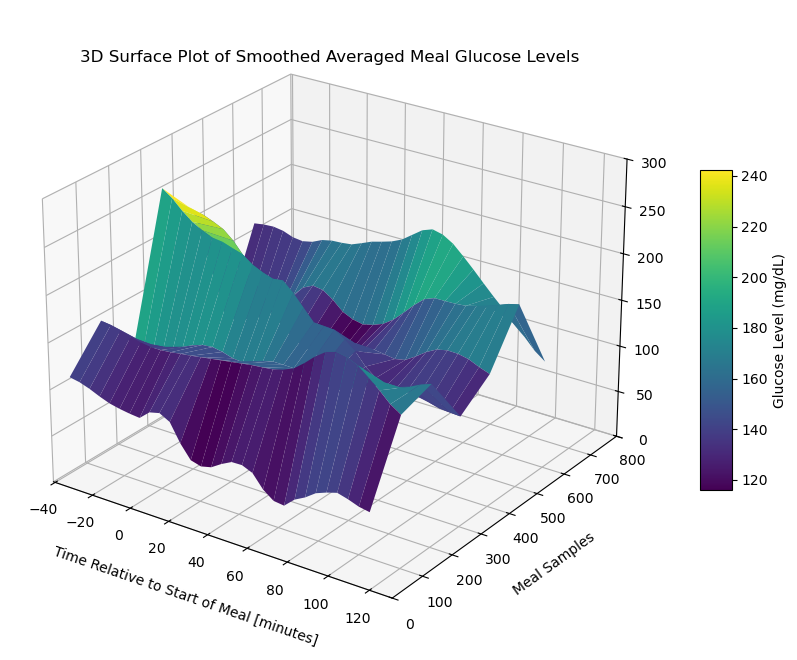
Contour Plot of Cleaned Imputed Meal Data Matrix 1
# Create the contour plot
plt.figure(figsize=(15, 10))
plt.contourf(X, Y, meal_data_matrix_1_df, cmap='viridis', levels=30)
plt.colorbar(label='Glucose Level (mg/dL)')
plt.title('Contour Plot of Meal Glucose Levels')
plt.xlabel('Time Points')
plt.ylabel('Meal Samples')
plt.show()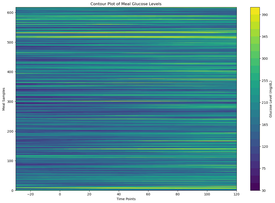
Visualize Cleaned Imputed Meal Data Matrix 2
Heatmap of Cleaned Imputed Meal Data Matrix 2
# Create the heatmap
sampled_meal_data_matrix_2 = cleaned_imputed_meal_matrix_1[np.random.choice(cleaned_imputed_meal_matrix_2.shape[0], 200, replace=False)]
plt.figure(figsize=(30, 30))
sns.heatmap(sampled_meal_data_matrix_2, cmap='YlGnBu', linewidths=0.5, annot=False, vmin=None, vmax=None)
plt.title('Heatmap of Meal Data Matrix 1')
plt.xlabel('Time Points')
plt.ylabel('Meals (Samples)')
plt.show()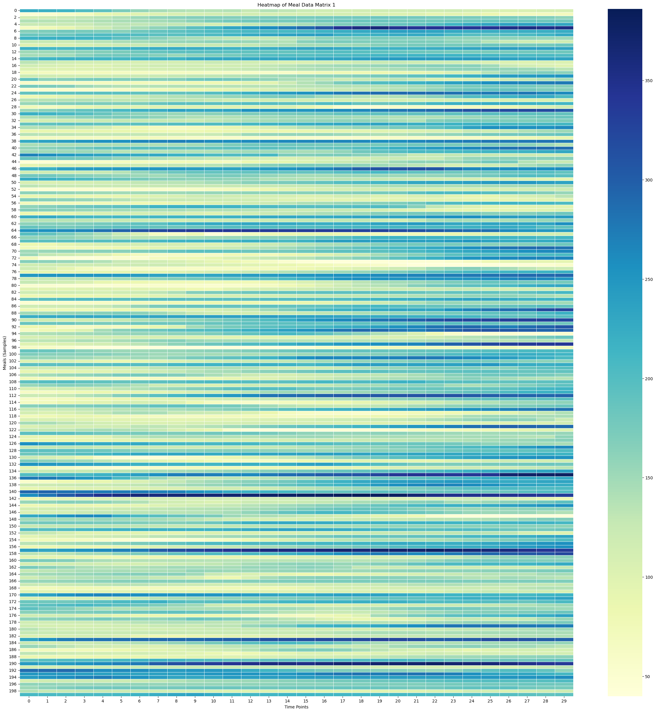
Surface Plot of Cleaned Imputed Meal Data Matrix 2
# Create X, Y meshgrid
X = np.arange(cleaned_imputed_meal_matrix_2.shape[1])
Y = np.arange(cleaned_imputed_meal_matrix_2.shape[0])
time_points = np.linspace(-30, 120, 30)  # X-axis: from -30 minutes to +120 minutes (30 time points)
meal_numbers = np.arange(1, len(meal_data_2) + 1)
X, Y = np.meshgrid(time_points, Y)
#X, Y = np.meshgrid(time_points, meal_numbers)Xarray([[-30. , -24.82758621, -19.65517241, ..., 109.65517241,
114.82758621, 120. ],
[-30. , -24.82758621, -19.65517241, ..., 109.65517241,
114.82758621, 120. ],
[-30. , -24.82758621, -19.65517241, ..., 109.65517241,
114.82758621, 120. ],
...,
[-30. , -24.82758621, -19.65517241, ..., 109.65517241,
114.82758621, 120. ],
[-30. , -24.82758621, -19.65517241, ..., 109.65517241,
114.82758621, 120. ],
[-30. , -24.82758621, -19.65517241, ..., 109.65517241,
114.82758621, 120. ]])X.shape(325, 30)Yarray([[ 0, 0, 0, ..., 0, 0, 0],
[ 1, 1, 1, ..., 1, 1, 1],
[ 2, 2, 2, ..., 2, 2, 2],
...,
[322, 322, 322, ..., 322, 322, 322],
[323, 323, 323, ..., 323, 323, 323],
[324, 324, 324, ..., 324, 324, 324]])# Fill NaNs using forward fill, then backward fill
meal_data_matrix_2_df = pd.DataFrame(cleaned_imputed_meal_matrix_2)
meal_data_matrix_2_filled = meal_data_matrix_2_df.ffill().bfill().values# Apply a moving average smoothing to each row
window_size = 3 # Choose a window size for smoothing
smoothed_meal_data_matrix_2 = np.array([uniform_filter1d(row, size=window_size) for row in meal_data_matrix_2_filled])# Create the plot
fig = plt.figure(figsize=(10, 8))
ax = fig.add_subplot(111, projection='3d')
stride = 100
# Plot the surface
surface_plot = ax.plot_surface(X[::stride], Y[::stride], smoothed_meal_data_matrix_2[::stride], cmap='viridis', edgecolor='none')
ax.set_title('3D Surface Plot of Smoothed Averaged Meal Glucose Levels', y=0.985)
ax.set_xlabel('Time Relative to Start of Meal [minutes]', labelpad=10)
ax.set_ylabel('Meal Samples', labelpad=10)
#ax.set_zlabel('Glucose Level (mg/dL)', labelpad=30)
#ax.set_xticks(np.linspace(-30, 120, 7))
# Adjust axis limits to create a zoom-out effect
#ax.set_xlim(-30, 120)
#ax.set_ylim(0, 800)
#ax.set_zlim(0, 300)
fig.colorbar(surface_plot, ax=ax, shrink=0.5, aspect=10, label='Glucose Level (mg/dL)')
#plt.tight_layout()
fig.subplots_adjust(left=0.01, right=1, top=0.9, bottom=0.1)
ax.view_init(elev=25, azim=-55)
plt.show()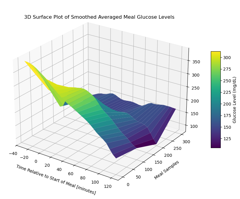
Contour Plot of Cleaned Imputed Meal Data Matrix 2
# Create the contour plot
plt.figure(figsize=(15, 10))
plt.contourf(X, Y, meal_data_matrix_2_df, cmap='viridis', levels=30)
plt.colorbar(label='Glucose Level (mg/dL)')
plt.title('Contour Plot of Meal Glucose Levels')
plt.xlabel('Time Points')
plt.ylabel('Meal Samples')
plt.show()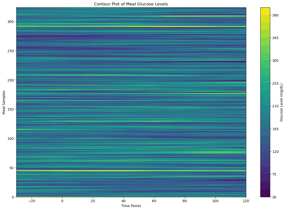
Combine Patient 1 and Patient 2 Data
cleaned_imputed_meal_matrix = \
    np.vstack((cleaned_imputed_meal_matrix_1, cleaned_imputed_meal_matrix_2))
cleaned_imputed_no_meal_matrix = \
np.vstack((cleaned_imputed_no_meal_matrix_1, cleaned_imputed_no_meal_matrix_2))Feature Extraction
Define Feature Extractor Helper Functions
def compute_first_derivative(glucose_data, delta_t=5):
    return np.diff(glucose_data) / delta_t
def compute_second_derivative(glucose_values, delta_t=5):
second_derivative = np.zeros(len(glucose_values) - 2)
for i in range(1, len(glucose_values) - 1):
second_derivative[i - 1] = \
(glucose_values[i + 1] - 2 * glucose_values[i] + glucose_values[i - 1]) / (delta_t ** 2)
return second_derivativecompute_first_derivative(cleaned_imputed_meal_matrix[0])array([-0.2 , -1. , -1. , -0.8 , -0.6 ,
0. , -0.4 , -0.25714286, 6.25714286, -4.4 ,
-5.4 , -1.6 , -1.6 , 1.4 , 1.8 ,
1. , 0.6 , -1.4 , -2. , -4.8 ,
1.8 , 2.2 , 2. , -0.62857143, 3.42857143,
-0.2 , -1.2 , -0.4 , -0.8 ])compute_second_derivative(cleaned_imputed_meal_matrix[0])array([-0.16 , 0. , 0.04 , 0.04 , 0.12 ,
-0.08 , 0.02857143, 1.30285714, -2.13142857, -0.2 ,
0.76 , 0. , 0.6 , 0.08 , -0.16 ,
-0.08 , -0.4 , -0.12 , -0.56 , 1.32 ,
0.08 , -0.04 , -0.52571429, 0.81142857, -0.72571429,
-0.2 , 0.16 , -0.08 ])def compute_AUC(glucose_values, delta_t=5):
return simpson(glucose_values, dx=delta_t)Define Feature Extractor Function
def feature_extractor(data_matrix):

    features = []

    for row in data_matrix:
        mean_glucose = np.mean(row)
        std_glucose  = np.std(row)
        max_glucose  = np.max(row)
        min_glucose  = np.min(row)

        first_derivative = compute_first_derivative(row)
        mean_first_derivate = np.mean(first_derivative)

        if len(row) > 2:
            second_derivative = compute_second_derivative(row)
            mean_second_derivative = np.mean(second_derivative)
        else:
            mean_second_derivative = 0

        AUC = compute_AUC(row)

        time_to_peak = np.argmax(row)

        features_vector = [
            mean_glucose,
            std_glucose,
            max_glucose,
            min_glucose,
            mean_first_derivate,
            mean_second_derivative,
            AUC,
            time_to_peak
        ]

        features.append(features_vector)

    return np.array(features)
Get Feature Matrix for Cleaned Imputed Meal Data
meal_features_matrix = feature_extractor(cleaned_imputed_meal_matrix)
meal_features_matrix[0]
array([ 8.98190476e+01, 1.91175360e+01, 1.31000000e+02, 4.90000000e+01,
-2.82758621e-01, -4.28571429e-03, 1.30310714e+04, 9.00000000e+00])Get Feature Matrix for Clean Imputed No Meal Data
no_meal_features_matrix = feature_extractor(cleaned_imputed_no_meal_matrix)
no_meal_features_matrix[0]
array([ 9.11607143e+01, 2.10808822e+01, 1.31000000e+02, 4.90000000e+01,
-3.65217391e-01, 2.00000000e-02, 1.04699405e+04, 9.00000000e+00])Visualize The Meal Features Matrix
Normalize The Data
scaler = StandardScaler()
scaled_meal_features_matrix = scaler.fit_transform(meal_features_matrix)
scaled_no_meal_features_matrix = scaler.fit_transform(no_meal_features_matrix)scaled_meal_features_matrix[0]array([-1.43931653, -0.6890434 , -1.43186426, -1.35409331, -0.73789252,
-0.2568468 , -1.42698567, -0.72547238])scaled_no_meal_features_matrix[0]array([-1.24861858, -0.24758492, -1.16121642, -1.39218291, -0.66468096,
1.06439767, -1.24077771, -0.41467362])Plot Features for all Rows
meal_features_matrix.shape[0]944X = np.arange(
start=0,
stop=meal_features_matrix.shape[0]
)Plot Max, Mean, Min, and Std Dev for All Rows
Y_mean = meal_features_matrix[:, 0] # First column
Y_mean_peaks, _ = find_peaks(Y_mean, height=20)

Y_mean_peaks_times = X[Y_mean_peaks]
Y_mean_peaks_values = Y_mean[Y_mean_peaks]

window_size = 3
Y_mean_peaks_moving_avg = np.convolve(Y_mean_peaks_values, np.ones(window_size)/window_size, mode='valid')
Y_std = meal_features_matrix[:, 1] # Second columnY_max = meal_features_matrix[:, 2] # Third column
Y_max_peaks, _ = find_peaks(Y_max, height=20)
Y_max_peaks_times = X[Y_max_peaks]
Y_max_peaks_values = Y_max[Y_max_peaks]
window_size = 3
Y_max_peaks_moving_avg = np.convolve(Y_max_peaks_values, np.ones(window_size)/window_size, mode='valid')Y_max_peaks_times.shape(289,)Y_max_peaks_moving_avg.shape(287,)Y_min = meal_features_matrix[:, 3] # Fourth column
Y_min_peaks, _ = find_peaks(Y_min, height=20)
Y_min_peaks_times = X[Y_min_peaks]
Y_min_peaks_values = Y_min[Y_min_peaks]
window_size = 3
Y_min_peaks_moving_avg = np.convolve(Y_min_peaks_values, np.ones(window_size)/window_size, mode='valid')Y_min_peaks_moving_avg.shape(281,)# Create the plot
fig = plt.figure(figsize=(18, 6))
ax = fig.add_subplot(111)
stride = 5
# Plot the features
#ax.plot(X[::stride], Y_max[::stride], 'x', label='Max', color='red')
ax.plot(Y_max_peaks_times[:len(Y_max_peaks_moving_avg)], Y_max_peaks_moving_avg, color='red', label='Moving Average of Max', linewidth=2)
#ax.plot(X[::stride], Y_mean[::stride], label='Mean', color='blue')
ax.plot(Y_mean_peaks_times[:len(Y_mean_peaks_moving_avg)], Y_mean_peaks_moving_avg, color='blue', label='Moving Average of Mean', linewidth=2)
#ax.plot(X[::stride], Y_min[::stride], 'x', label='Min')
ax.plot(Y_min_peaks_times[:len(Y_min_peaks_moving_avg)], Y_min_peaks_moving_avg, color='green', label='Moving Average of Min', linewidth=2)
ax.plot(X[::stride], Y_std[::stride], label='Std Dev')
ax.set_title('Meal Glucose Level Features vs Data Row Number', fontsize=20)
ax.set_xlabel('Data Row Number [arbitrary] ', fontsize=16)
ax.set_ylabel('Glucose Level [mg/dL]', fontsize=16)
ax.set_xticks(np.linspace(0, 1000, 11))
ax.set_yticks(np.linspace(0, 400, 7))
ax.set_xlim(-50, 1000)
ax.set_ylim(0, 420)
#ax.text(300, 380, f'Viewing every {stride} rows')
# Adjust axis limits to create a zoom-out effect
#ax.set_xlim(-30, 120)
#ax.set_ylim(0, 800)
#plt.tight_layout()
plt.legend()
plt.show()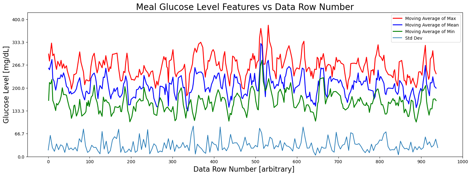
Plot First and Second Derivatives
Y_mean_first_derivative = meal_features_matrix[:, 4] # Fourth column
Y_mean_first_derivative_peaks, _ = find_peaks(Y_mean_first_derivative, height=None)

Y_mean_first_derivative_times = X[Y_mean_first_derivative_peaks]
Y_mean_first_derivative_values = Y_mean_first_derivative[Y_mean_first_derivative_peaks]

window_size = 3
Y_mean_first_derivative_peaks_moving_avg = \
    np.convolve(
        Y_mean_first_derivative_values,
        np.ones(window_size)/window_size, mode='valid'
    )
Y_mean_2nd_derivative = meal_features_matrix[:, 5] # Fourth column
Y_mean_2nd_derivative_peaks, _ = find_peaks(Y_mean_2nd_derivative, height=None)
Y_mean_2nd_derivative_times = X[Y_mean_2nd_derivative_peaks]
Y_mean_2nd_derivative_values = Y_mean_2nd_derivative[Y_mean_2nd_derivative_peaks]
window_size = 3
Y_mean_2nd_derivative_peaks_moving_avg = \
np.convolve(
Y_mean_2nd_derivative_values,
np.ones(window_size)/window_size, mode='valid'
)# Create the plot
fig = plt.figure(figsize=(18, 6))
ax = fig.add_subplot(111)
stride = 5
# Plot the features
#ax.plot(X[::stride], Y_max[::stride], 'x', label='Max', color='red')
#ax.plot(
# Y_max_peaks_times[:len(Y_max_peaks_moving_avg)],
# Y_max_peaks_moving_avg,
# color='red',
# label='Moving Average of Max',
# linewidth=2)
#ax.plot(X[::stride], Y_mean[::stride], label='Mean', color='blue')
ax.plot(
Y_mean_peaks_times[:len(Y_mean_peaks_moving_avg)],
Y_mean_peaks_moving_avg,
color='blue',
label='Moving Average of Mean',
linewidth=2
)
#ax.plot(X[::stride], Y_min[::stride], 'x', label='Min')
#ax.plot(Y_min_peaks_times[:len(Y_min_peaks_moving_avg)], Y_min_peaks_moving_avg, color='green', label='Moving Average of Min', linewidth=2)
#ax.plot(X[::stride], Y_std[::stride], label='Std Dev')
ax.plot(
Y_mean_first_derivative_times[:len(Y_mean_first_derivative_peaks_moving_avg)],
Y_mean_first_derivative_peaks_moving_avg*100,
color='orange',
label=r'First Derivative $\times 100$',
linewidth=2
)
ax.plot(
Y_mean_2nd_derivative_times[:len(Y_mean_2nd_derivative_peaks_moving_avg)],
Y_mean_2nd_derivative_peaks_moving_avg*2500,
color='green',
label=r'Second Derivative $\times 2500$',
linewidth=2
)
ax.set_title('Glucose Level Features vs Data Row Number')
ax.set_xlabel('Data Row Number [arbitrary] ')
ax.set_ylabel('Glucose Level [mg/dL]')
#ax.set_xticks(np.linspace(0, 1000, 11))
#ax.set_yticks(np.linspace(0, 400, 7))
#ax.set_xlim(-50, 1000)
#ax.set_ylim(0, 420)
#ax.text(300, 380, f'Viewing every {stride} rows')
# Adjust axis limits to create a zoom-out effect
#ax.set_xlim(-30, 120)
#ax.set_ylim(0, 800)
#plt.tight_layout()
plt.legend()
plt.show()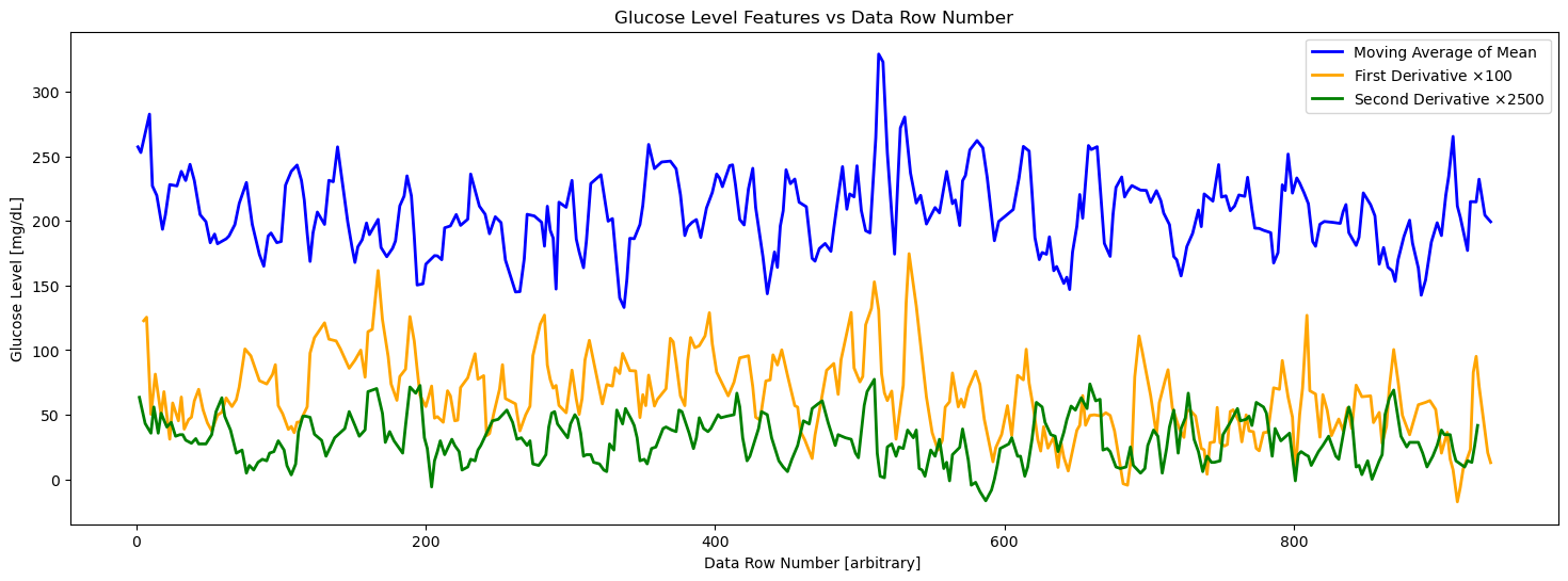
Pairwise Plot of Meal Features Matrix
# Generate column labels for the features
feature_columns = [f'Feature_{i+1}' for i in range(meal_features_matrix.shape[1])]

# Convert the feature matrix to a Pandas DataFrame
df = pd.DataFrame(meal_features_matrix, columns=feature_columns)

# Create a pairwise plot using Seaborn
plt.figure(figsize=(15, 15))  # Adjust figure size as needed
sns.pairplot(df, diag_kind='hist', plot_kws={'alpha': 0.5, 's': 40})

plt.suptitle('Pairwise Plot of Meal Features Matrix', y=1.02, fontsize=30)

# Show the plot
plt.show()
<Figure size 1500x1500 with 0 Axes>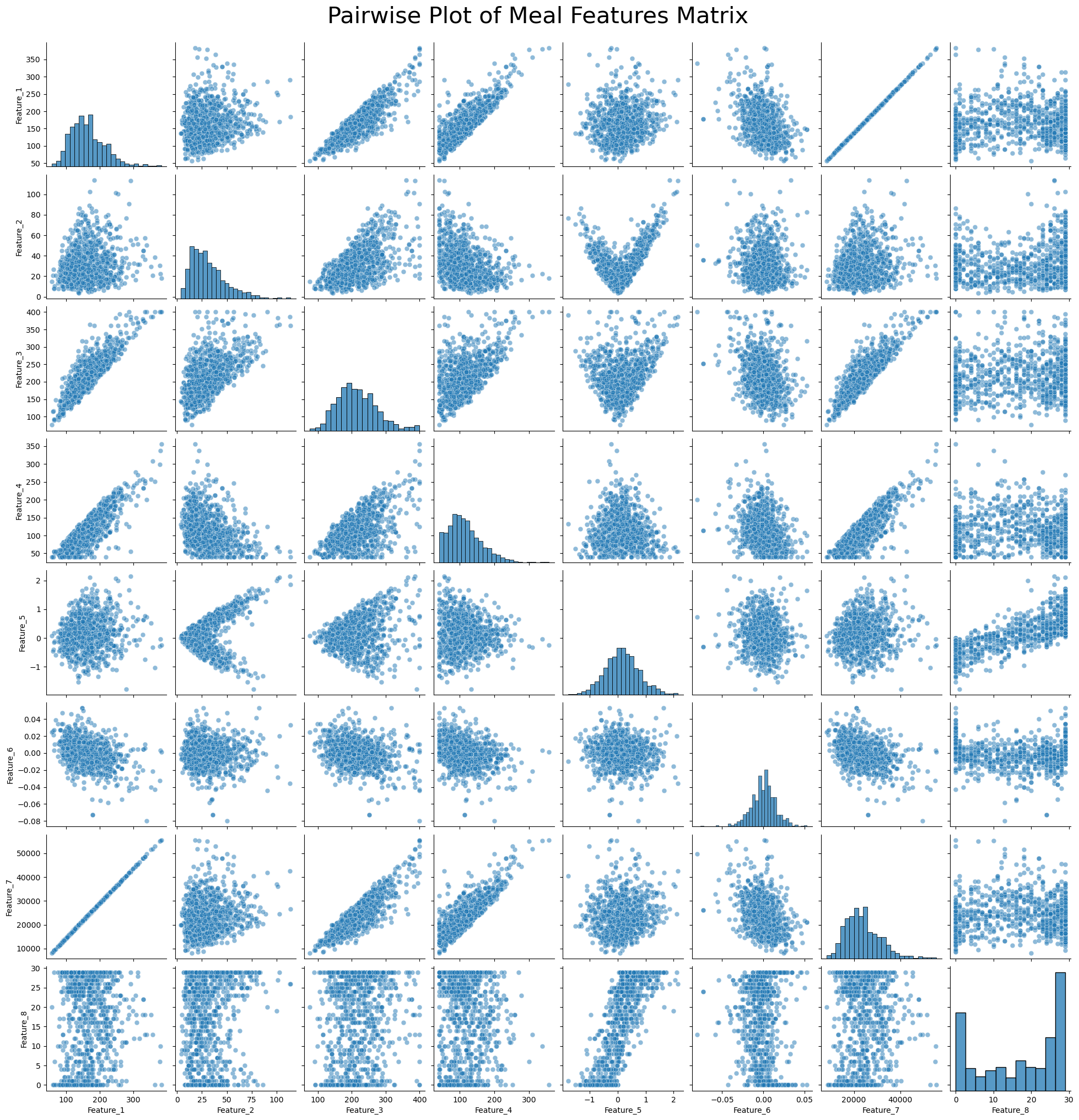
Visualize The No Meal Features Matrix
Normalize The Data
scaler = StandardScaler()
scaled_meal_features_matrix = scaler.fit_transform(meal_features_matrix)
scaled_no_meal_features_matrix = scaler.fit_transform(no_meal_features_matrix)scaled_meal_features_matrix[0]array([-1.43931653, -0.6890434 , -1.43186426, -1.35409331, -0.73789252,
-0.2568468 , -1.42698567, -0.72547238])scaled_no_meal_features_matrix[0]array([-1.24861858, -0.24758492, -1.16121642, -1.39218291, -0.66468096,
1.06439767, -1.24077771, -0.41467362])Plot Features for all Rows
no_meal_features_matrix.shape[0]752X = np.arange(
start=0,
stop=no_meal_features_matrix.shape[0]
)Plot Max, Mean, Min, and Std Dev for All Rows
Y_mean = no_meal_features_matrix[:, 0] # First column
Y_mean_peaks, _ = find_peaks(Y_mean, height=20)

Y_mean_peaks_times = X[Y_mean_peaks]
Y_mean_peaks_values = Y_mean[Y_mean_peaks]

window_size = 3
Y_mean_peaks_moving_avg = np.convolve(Y_mean_peaks_values, np.ones(window_size)/window_size, mode='valid')
Y_std = no_meal_features_matrix[:, 1] # Second columnY_max = no_meal_features_matrix[:, 2] # Third column
Y_max_peaks, _ = find_peaks(Y_max, height=20)
Y_max_peaks_times = X[Y_max_peaks]
Y_max_peaks_values = Y_max[Y_max_peaks]
window_size = 3
Y_max_peaks_moving_avg = np.convolve(Y_max_peaks_values, np.ones(window_size)/window_size, mode='valid')Y_max_peaks_times.shape(238,)Y_max_peaks_moving_avg.shape(236,)Y_min = no_meal_features_matrix[:, 3] # Fourth column
Y_min_peaks, _ = find_peaks(Y_min, height=20)
Y_min_peaks_times = X[Y_min_peaks]
Y_min_peaks_values = Y_min[Y_min_peaks]
window_size = 3
Y_min_peaks_moving_avg = np.convolve(Y_min_peaks_values, np.ones(window_size)/window_size, mode='valid')Y_min_peaks_moving_avg.shape(238,)# Create the plot
fig = plt.figure(figsize=(18, 6))
ax = fig.add_subplot(111)
stride = 5
# Plot the features
#ax.plot(X[::stride], Y_max[::stride], 'x', label='Max', color='red')
ax.plot(Y_max_peaks_times[:len(Y_max_peaks_moving_avg)], Y_max_peaks_moving_avg, color='red', label='Moving Average of Max', linewidth=2)
#ax.plot(X[::stride], Y_mean[::stride], label='Mean', color='blue')
ax.plot(Y_mean_peaks_times[:len(Y_mean_peaks_moving_avg)], Y_mean_peaks_moving_avg, color='blue', label='Moving Average of Mean', linewidth=2)
#ax.plot(X[::stride], Y_min[::stride], 'x', label='Min')
ax.plot(Y_min_peaks_times[:len(Y_min_peaks_moving_avg)], Y_min_peaks_moving_avg, color='green', label='Moving Average of Min', linewidth=2)
ax.plot(X[::stride], Y_std[::stride], label='Std Dev')
ax.set_title('No Meal Glucose Level Features vs Data Row Number', fontsize=20)
ax.set_xlabel('Data Row Number [arbitrary] ', fontsize=16)
ax.set_ylabel('Glucose Level [mg/dL]', fontsize=16)
ax.set_xticks(np.linspace(0, 800, 11))
ax.set_yticks(np.linspace(0, 400, 7))
ax.set_xlim(-50, 800)
ax.set_ylim(0, 420)
#ax.text(300, 380, f'Viewing every {stride} rows')
# Adjust axis limits to create a zoom-out effect
#ax.set_xlim(-30, 120)
#ax.set_ylim(0, 800)
#plt.tight_layout()
plt.legend()
plt.show()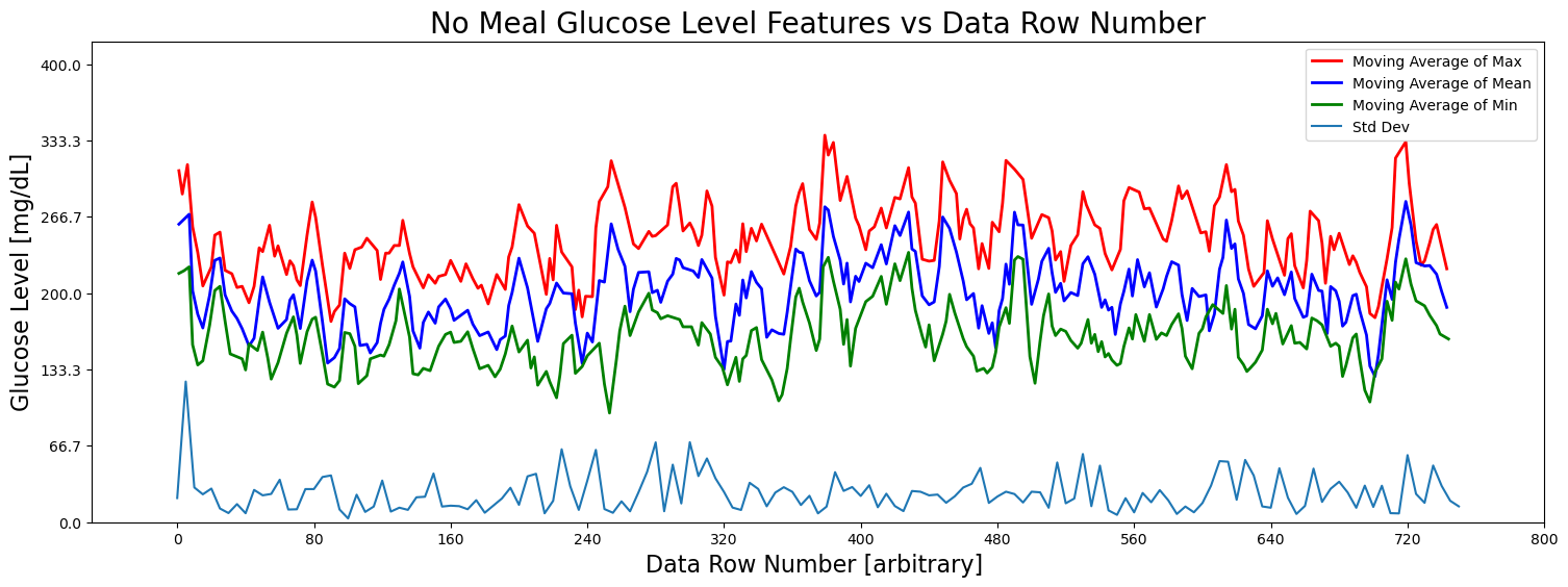
Pairwise Plot of No Meal Features Matrix
# Generate column labels for the features
feature_columns = [f'Feature_{i+1}' for i in range(meal_features_matrix.shape[1])]

# Convert the feature matrix to a Pandas DataFrame
df = pd.DataFrame(no_meal_features_matrix, columns=feature_columns)

# Create a pairwise plot using Seaborn
plt.figure(figsize=(15, 15))  # Adjust figure size as needed
sns.pairplot(df, diag_kind='hist', plot_kws={'alpha': 0.5, 's': 40})

plt.suptitle('Pairwise Plot of No Meal Features Matrix', y=1.02, fontsize=30)

# Show the plot
plt.show()
<Figure size 1500x1500 with 0 Axes>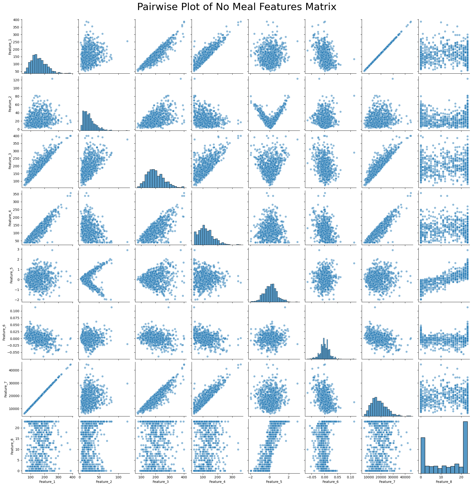
Concatenate Feature Matrices and Add Class Labels
meal_labels = np.ones((meal_features_matrix.shape[0], 1))
len(meal_labels)944meal_features_matrix_with_labels = \
np.hstack((meal_features_matrix, meal_labels))
#meal_features_matrix_with_labels[1]no_meal_labels = np.zeros((no_meal_features_matrix.shape[0], 1))
len(no_meal_labels)752no_meal_features_matrix_with_labels = \
np.hstack((no_meal_features_matrix, no_meal_labels))
#no_meal_features_matrix_with_labels[1]concat_features = \
np.vstack((meal_features_matrix_with_labels, no_meal_features_matrix_with_labels))
len(concat_features)1696Train Support Vector Machine
Use Standard Variable Names for Features and Class Label
X = concat_features[:, :-1]
y = concat_features[:, -1]X[0]array([ 8.98190476e+01, 1.91175360e+01, 1.31000000e+02, 4.90000000e+01,
-2.82758621e-01, -4.28571429e-03, 1.30310714e+04, 9.00000000e+00])y[0]np.float64(1.0)Train / Test Split
X_train, X_test, y_train, y_test = \
    train_test_split(X, y, test_size = 0.2, random_state=40)
Normalize The Data
scaler = StandardScaler()
X_train_scaled = scaler.fit_transform(X_train)
X_test_scaled = scaler.fit_transform(X_test)
Train SVM Model
svm_model = SVC(kernel='linear', C=0.1)
svm_model.fit(X_train_scaled, y_train)
Loading...
Test SVM Model
y_pred = svm_model.predict(X_test_scaled)Obtain Accuracy of SVM Model
accuracy = accuracy_score(y_test, y_pred)
print(f"Accuracy: {accuracy * 100:.2f}%")
Accuracy: 99.71%
Obtain Training and Test Accuracy of SVM Model
train_accuracy = svm_model.score(X_train_scaled, y_train)
test_accuracy = svm_model.score(X_test_scaled, y_test)
print(f"Training Accuracy: {train_accuracy * 100:.2f}%")
print(f"Test Accuracy: {test_accuracy * 100:.2f}%")
Training Accuracy: 100.00%
Test Accuracy: 99.71%
Obtain F1 Score of SVM Model
f1 = f1_score(y_test, y_pred)
print(f"F1 Score: {f1:.2f}")
F1 Score: 1.00
Cross Validate SVM Model
scores = cross_val_score(svm_model, X_train_scaled, y_train, cv=5, scoring='accuracy')
print(f"Cross-Validation Accuracy: {scores.mean():.2f} (+/- {scores.std():.2f})")
Cross-Validation Accuracy: 1.00 (+/- 0.00)
Visualize Results of SVM Model
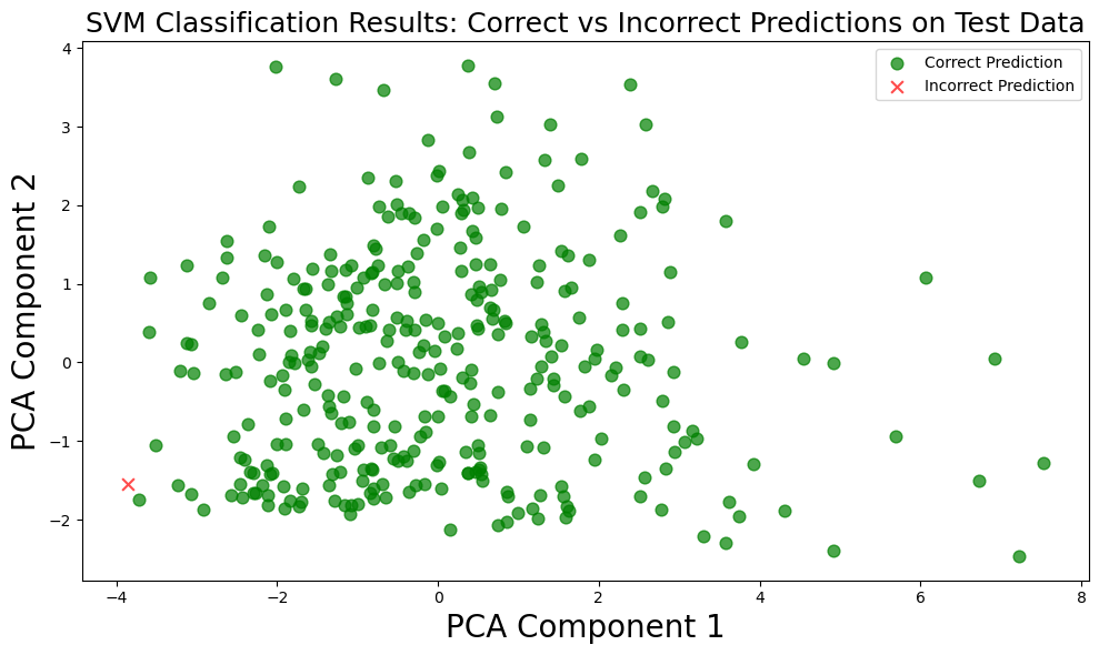
Scatter Plot with PCA
# Reduce dimensions using PCA
pca = PCA(n_components=2)

X_reduced = pca.fit_transform(X_test_scaled)

components = pca.components_
print(components)

# Get the predicted labels
predicted_labels = svm_model.predict(X_test_scaled)

# Create boolean masks for correct and incorrect predictions
correct_mask = (predicted_labels == y_test)
incorrect_mask = ~correct_mask

# Create a figure
plt.figure(figsize=(10, 6))

# Plot correct predictions in green
plt.scatter(X_reduced[correct_mask, 0], X_reduced[correct_mask, 1], color='green',
            marker='o', alpha=0.7, s=60, label='Correct Prediction')

# Plot incorrect predictions in red
plt.scatter(X_reduced[incorrect_mask, 0], X_reduced[incorrect_mask, 1], color='red',
            marker='x', alpha=0.7, s=60, label='Incorrect Prediction')

# Set labels and title
plt.xlabel('PCA Component 1', fontsize=20)
plt.ylabel('PCA Component 2', fontsize=20)
plt.title('SVM Classification Results: Correct vs Incorrect Predictions on Test Data', fontsize=18)

# Add a legend
plt.legend()

# Display the plot
plt.tight_layout()
plt.show()
[[ 0.51111341 0.13118439 0.47327076 0.4251986 0.00643744 -0.257121
0.50031459 0.01753109]
[-0.03692307 0.31993471 0.1095569 -0.19047139 0.66528982 0.06390289
0.01416038 0.63332595]]
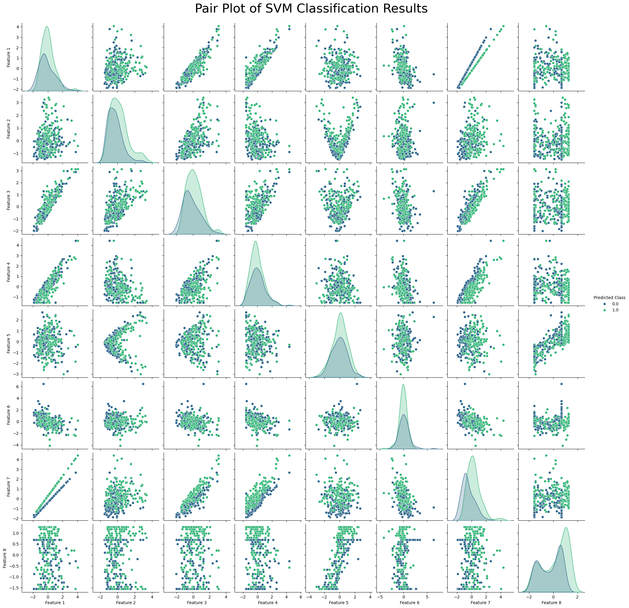
Pairwise Plotting of Feature vs Feature
df = pd.DataFrame(X_test_scaled, columns=[f'Feature {i+1}' for i in range(X_test_scaled.shape[1])])
df['Predicted Class'] = svm_model.predict(X_test_scaled)

# Plot pairwise relationships
sns.pairplot(df, hue='Predicted Class', palette='viridis')
plt.suptitle('Pair Plot of SVM Classification Results', y=1.02, fontsize=30)
plt.show()
Heatmaps of Confusion Matrix
# Get the predicted classes
y_pred = svm_model.predict(X_test_scaled)

# Create the confusion matrix
cm = confusion_matrix(y_test, y_pred)

# Plot the heatmap of the confusion matrix
sns.heatmap(cm, annot=True, cmap='Blues', fmt='d')
plt.xlabel('Predicted')
plt.ylabel('Actual')
plt.title('Confusion Matrix Heatmap of Test Data')
plt.show()


# Print accuracy, recall, precision, and F1 score
accuracy = accuracy_score(y_test, y_pred)
recall = recall_score(y_test, y_pred)
precision = precision_score(y_test, y_pred)
f1 = f1_score(y_test, y_pred)

print(f'Accuracy: {accuracy:.4f}')
print(f'Recall: {recall:.4f}')
print(f'Precision: {precision:.4f}')
print(f'F1 Score: {f1:.4f}')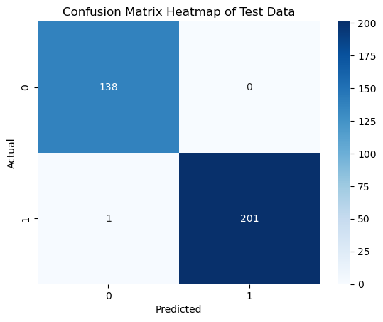
Accuracy: 0.9971
Recall: 0.9950
Precision: 1.0000
F1 Score: 0.9975
Dump Model to Pickle File
with open('svm_model.pkl', 'wb') as f:
    pickle.dump(svm_model, f)