"""
Created on Mon Apr 15 19:43:04 2019

Updated on Wed Jan 29 10:18:09 2020

@author: created by Sowmya Myneni and updated by Dijiang Huang
"""
'\nCreated on Mon Apr 15 19:43:04 2019\n\nUpdated on Wed Jan 29 10:18:09 2020\n\n@author: created by Sowmya Myneni and updated by Dijiang Huang\n'import matplotlib.pyplot as plt
import tensorflow as tf
print("Num GPUs Available:", len(tf.config.list_physical_devices('GPU')))2024-12-06 10:45:02.246067: I tensorflow/core/platform/cpu_feature_guard.cc:210] This TensorFlow binary is optimized to use available CPU instructions in performance-critical operations.
To enable the following instructions: SSE4.1 SSE4.2, in other operations, rebuild TensorFlow with the appropriate compiler flags.
Num GPUs Available: 0
import os
import multiprocessing

# Number of logical CPUs
num_cores = multiprocessing.cpu_count()
print(f"Number of CPU cores available: {num_cores}")
Number of CPU cores available: 12
# Configure TensorFlow to use all available CPU cores
tf.config.threading.set_intra_op_parallelism_threads(0)  # Use all intra-operation threads
tf.config.threading.set_inter_op_parallelism_threads(0)  # Use all inter-operation threads
FNN Sample SB
########################################
# Part 1 - Data Pre-Processing
#######################################

# To load a dataset file in Python, you can use Pandas. Import pandas using the line below
import pandas as pd
# Import numpy to perform operations on the dataset
import numpy as np
Variable Setup
# Variable Setup
# Available datasets: KDDTrain+.txt, KDDTest+.txt, etc. More read Data Set Introduction.html within the NSL-KDD dataset folder
# Type the training dataset file name in ''
#TrainingDataPath='NSL-KDD/'
#TrainingData='KDDTrain+_20Percent.txt'
# Batch Size
BatchSize=10
# Epohe Size
NumEpoch=10
Import Training Dataset
# Import dataset.
# Dataset is given in TraningData variable You can replace it with the file
# path such as “C:\Users\...\dataset.csv’.
# The file can be a .txt as well.
# If the dataset file has header, then keep header=0 otherwise use header=none
# reference: https://www.shanelynn.ie/select-pandas-dataframe-rows-and-columns-using-iloc-loc-and-ix/
dataset_train = pd.read_csv('Training-a1-a2.csv', header=None)dataset_train.info()<class 'pandas.core.frame.DataFrame'>
RangeIndex: 124926 entries, 0 to 124925
Data columns (total 43 columns):
# Column Non-Null Count Dtype
--- ------ -------------- -----
0 0 124926 non-null int64
1 1 124926 non-null object
2 2 124926 non-null object
3 3 124926 non-null object
4 4 124926 non-null int64
5 5 124926 non-null int64
6 6 124926 non-null int64
7 7 124926 non-null int64
8 8 124926 non-null int64
9 9 124926 non-null int64
10 10 124926 non-null int64
11 11 124926 non-null int64
12 12 124926 non-null int64
13 13 124926 non-null int64
14 14 124926 non-null int64
15 15 124926 non-null int64
16 16 124926 non-null int64
17 17 124926 non-null int64
18 18 124926 non-null int64
19 19 124926 non-null int64
20 20 124926 non-null int64
21 21 124926 non-null int64
22 22 124926 non-null int64
23 23 124926 non-null int64
24 24 124926 non-null float64
25 25 124926 non-null float64
26 26 124926 non-null float64
27 27 124926 non-null float64
28 28 124926 non-null float64
29 29 124926 non-null float64
30 30 124926 non-null float64
31 31 124926 non-null int64
32 32 124926 non-null int64
33 33 124926 non-null float64
34 34 124926 non-null float64
35 35 124926 non-null float64
36 36 124926 non-null float64
37 37 124926 non-null float64
38 38 124926 non-null float64
39 39 124926 non-null float64
40 40 124926 non-null float64
41 41 124926 non-null object
42 42 124926 non-null int64
dtypes: float64(15), int64(24), object(4)
memory usage: 41.0+ MB
dataset_train.describe()Loading...
# Identify the column that contains the attack types
# Assuming the column with attack types is named based on the sample data ("neptune", "normal", etc.)
attack_column = dataset_train.columns[-2]  # Second last column seems to have attack types

# Calculate the frequency of each attack type
attack_distribution = dataset_train[attack_column].value_counts()

plt.figure(figsize=(10, 6))
attack_distribution.plot(kind='bar', logy=True)
plt.title('A1 and A2 Training Dataset Distribution of Attack Types')
plt.xlabel('Attack Type')
plt.ylabel('Frequency')
plt.xticks(rotation=45)
plt.tight_layout()
plt.show()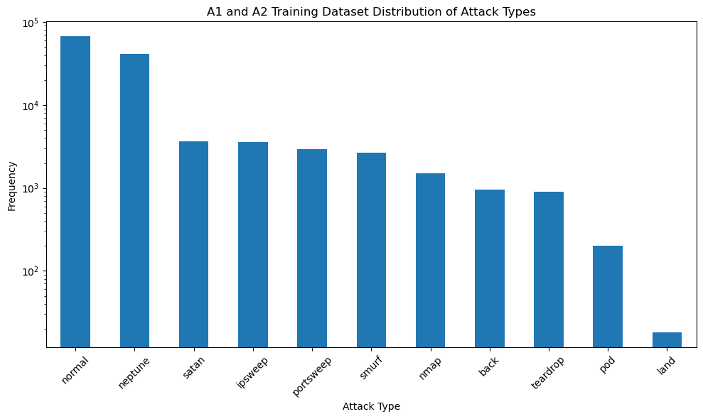
X_train = dataset_train.iloc[:, 0:-2].values
X_train
array([[0, 'tcp', 'ftp_data', ..., 0.0, 0.05, 0.0],
[0, 'udp', 'other', ..., 0.0, 0.0, 0.0],
[0, 'tcp', 'private', ..., 1.0, 0.0, 0.0],
...,
[0, 'tcp', 'smtp', ..., 0.0, 0.01, 0.0],
[0, 'tcp', 'klogin', ..., 1.0, 0.0, 0.0],
[0, 'tcp', 'ftp_data', ..., 0.0, 0.0, 0.0]], dtype=object)X_train.shape(124926, 41)label_column_train = dataset_train.iloc[:, -2].values
label_column_trainarray(['normal', 'normal', 'neptune', ..., 'normal', 'neptune', 'normal'],
dtype=object)y_train = []
for i in range(len(label_column_train)):
if label_column_train[i] == 'normal':
y_train.append(0)
else:
y_train.append(1)
# Convert list to array
y_train = np.array(y_train)y_trainarray([0, 0, 1, ..., 0, 1, 0])y_train.shape(124926,)Import Testing Dataset
# Import dataset.
# Dataset is given in TraningData variable You can replace it with the file
# path such as “C:\Users\...\dataset.csv’.
# The file can be a .txt as well.
# If the dataset file has header, then keep header=0 otherwise use header=none
# reference: https://www.shanelynn.ie/select-pandas-dataframe-rows-and-columns-using-iloc-loc-and-ix/
dataset_test = pd.read_csv('Testing-a1.csv', header=None)dataset_test.info()<class 'pandas.core.frame.DataFrame'>
RangeIndex: 17171 entries, 0 to 17170
Data columns (total 43 columns):
# Column Non-Null Count Dtype
--- ------ -------------- -----
0 0 17171 non-null int64
1 1 17171 non-null object
2 2 17171 non-null object
3 3 17171 non-null object
4 4 17171 non-null int64
5 5 17171 non-null int64
6 6 17171 non-null int64
7 7 17171 non-null int64
8 8 17171 non-null int64
9 9 17171 non-null int64
10 10 17171 non-null int64
11 11 17171 non-null int64
12 12 17171 non-null int64
13 13 17171 non-null int64
14 14 17171 non-null int64
15 15 17171 non-null int64
16 16 17171 non-null int64
17 17 17171 non-null int64
18 18 17171 non-null int64
19 19 17171 non-null int64
20 20 17171 non-null int64
21 21 17171 non-null int64
22 22 17171 non-null int64
23 23 17171 non-null int64
24 24 17171 non-null float64
25 25 17171 non-null float64
26 26 17171 non-null float64
27 27 17171 non-null float64
28 28 17171 non-null float64
29 29 17171 non-null float64
30 30 17171 non-null float64
31 31 17171 non-null int64
32 32 17171 non-null int64
33 33 17171 non-null float64
34 34 17171 non-null float64
35 35 17171 non-null float64
36 36 17171 non-null float64
37 37 17171 non-null float64
38 38 17171 non-null float64
39 39 17171 non-null float64
40 40 17171 non-null float64
41 41 17171 non-null object
42 42 17171 non-null int64
dtypes: float64(15), int64(24), object(4)
memory usage: 5.6+ MB
dataset_test.describe()Loading...
# Identify the column that contains the attack types
# Assuming the column with attack types is named based on the sample data ("neptune", "normal", etc.)
attack_column = dataset_test.columns[-2]  # Second last column seems to have attack types

# Calculate the frequency of each attack type
attack_distribution = dataset_test[attack_column].value_counts()

plt.figure(figsize=(10, 6))
attack_distribution.plot(kind='bar', logy=True)
plt.title('A1 Testing Dataset Distribution of Attack Types')
plt.xlabel('Attack Type')
plt.ylabel('Frequency')
plt.xticks(rotation=45)
plt.tight_layout()
plt.show()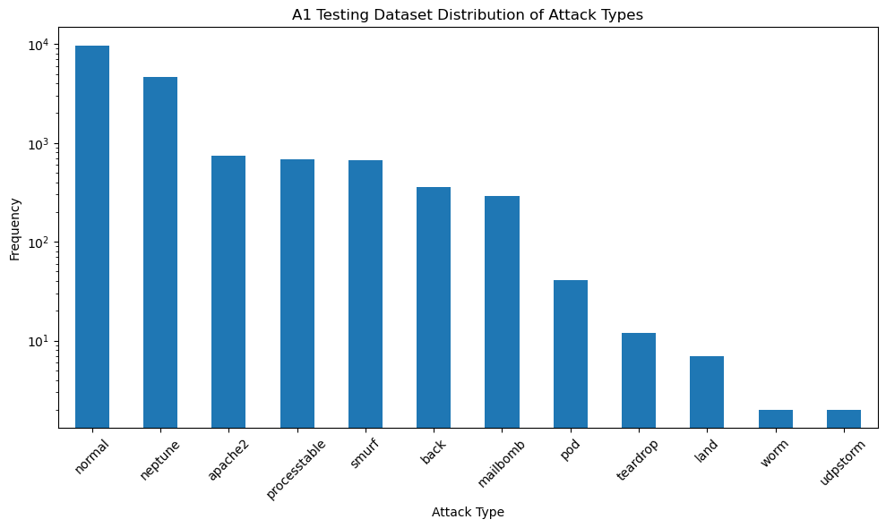
X_test = dataset_test.iloc[:, 0:-2].values
X_test
array([[0, 'tcp', 'private', ..., 0.0, 1.0, 1.0],
[0, 'tcp', 'private', ..., 0.0, 1.0, 1.0],
[2, 'tcp', 'ftp_data', ..., 0.0, 0.0, 0.0],
...,
[0, 'tcp', 'http', ..., 0.0, 0.0, 0.0],
[0, 'tcp', 'http', ..., 0.0, 0.07, 0.07],
[0, 'udp', 'domain_u', ..., 0.0, 0.0, 0.0]], dtype=object)X_test.shape(17171, 41)label_column_test = dataset_test.iloc[:, -2].values
label_column_testarray(['neptune', 'neptune', 'normal', ..., 'normal', 'back', 'normal'],
dtype=object)y_test = []
for i in range(len(label_column_test)):
if label_column_test[i] == 'normal':
y_test.append(0)
else:
y_test.append(1)
# Convert list to array
y_test = np.array(y_test)y_testarray([1, 1, 0, ..., 0, 1, 0])Encoding categorical data (convert letters/words in numbers)
# The following code work Python 3.7 or newer
from sklearn.preprocessing import OneHotEncoder
from sklearn.compose import ColumnTransformer
ct = ColumnTransformer(
     # The column numbers to be transformed ([1, 2, 3] represents three columns to be transferred)
    [('one_hot_encoder', OneHotEncoder(handle_unknown='ignore'), [1,2,3])],
    # Leave the rest of the columns untouched
    remainder='passthrough'
)
X_train = np.array(ct.fit_transform(X_train), dtype=np.float64)
X_test = np.array(ct.transform(X_test) , dtype=np.float64)X_trainarray([[0. , 1. , 0. , ..., 0. , 0.05, 0. ],
[0. , 0. , 1. , ..., 0. , 0. , 0. ],
[0. , 1. , 0. , ..., 1. , 0. , 0. ],
...,
[0. , 1. , 0. , ..., 0. , 0.01, 0. ],
[0. , 1. , 0. , ..., 1. , 0. , 0. ],
[0. , 1. , 0. , ..., 0. , 0. , 0. ]])X_train[0]array([0.00e+00, 1.00e+00, 0.00e+00, 0.00e+00, 0.00e+00, 0.00e+00,
0.00e+00, 0.00e+00, 0.00e+00, 0.00e+00, 0.00e+00, 0.00e+00,
0.00e+00, 0.00e+00, 0.00e+00, 0.00e+00, 0.00e+00, 0.00e+00,
0.00e+00, 0.00e+00, 0.00e+00, 0.00e+00, 0.00e+00, 1.00e+00,
0.00e+00, 0.00e+00, 0.00e+00, 0.00e+00, 0.00e+00, 0.00e+00,
0.00e+00, 0.00e+00, 0.00e+00, 0.00e+00, 0.00e+00, 0.00e+00,
0.00e+00, 0.00e+00, 0.00e+00, 0.00e+00, 0.00e+00, 0.00e+00,
0.00e+00, 0.00e+00, 0.00e+00, 0.00e+00, 0.00e+00, 0.00e+00,
0.00e+00, 0.00e+00, 0.00e+00, 0.00e+00, 0.00e+00, 0.00e+00,
0.00e+00, 0.00e+00, 0.00e+00, 0.00e+00, 0.00e+00, 0.00e+00,
0.00e+00, 0.00e+00, 0.00e+00, 0.00e+00, 0.00e+00, 0.00e+00,
0.00e+00, 0.00e+00, 0.00e+00, 0.00e+00, 0.00e+00, 0.00e+00,
0.00e+00, 0.00e+00, 0.00e+00, 0.00e+00, 0.00e+00, 0.00e+00,
0.00e+00, 0.00e+00, 0.00e+00, 0.00e+00, 1.00e+00, 0.00e+00,
0.00e+00, 4.91e+02, 0.00e+00, 0.00e+00, 0.00e+00, 0.00e+00,
0.00e+00, 0.00e+00, 0.00e+00, 0.00e+00, 0.00e+00, 0.00e+00,
0.00e+00, 0.00e+00, 0.00e+00, 0.00e+00, 0.00e+00, 0.00e+00,
0.00e+00, 2.00e+00, 2.00e+00, 0.00e+00, 0.00e+00, 0.00e+00,
0.00e+00, 1.00e+00, 0.00e+00, 0.00e+00, 1.50e+02, 2.50e+01,
1.70e-01, 3.00e-02, 1.70e-01, 0.00e+00, 0.00e+00, 0.00e+00,
5.00e-02, 0.00e+00])X_train.shape(124926, 122)X_testarray([[0. , 1. , 0. , ..., 0. , 1. , 1. ],
[0. , 1. , 0. , ..., 0. , 1. , 1. ],
[0. , 1. , 0. , ..., 0. , 0. , 0. ],
...,
[0. , 1. , 0. , ..., 0. , 0. , 0. ],
[0. , 1. , 0. , ..., 0. , 0.07, 0.07],
[0. , 0. , 1. , ..., 0. , 0. , 0. ]])X_test.shape(17171, 122)Perform feature scaling
# Perform feature scaling. For ANN you can use StandardScaler, for RNNs recommended is
# MinMaxScaler.
# referece: https://scikit-learn.org/stable/modules/generated/sklearn.preprocessing.StandardScaler.html
# https://scikit-learn.org/stable/modules/preprocessing.html
from sklearn.preprocessing import StandardScaler
sc = StandardScaler()
X_train = sc.fit_transform(X_train)  # Scaling to the range [0,1]
X_test = sc.fit_transform(X_test)X_trainarray([[-0.26661772, 0.47858359, -0.3692588 , ..., -0.6282041 ,
-0.225902 , -0.3774467 ],
[-0.26661772, -2.08949913, 2.70812776, ..., -0.6282041 ,
-0.38864593, -0.3774467 ],
[-0.26661772, 0.47858359, -0.3692588 , ..., 1.60987176,
-0.38864593, -0.3774467 ],
...,
[-0.26661772, 0.47858359, -0.3692588 , ..., -0.6282041 ,
-0.35609714, -0.3774467 ],
[-0.26661772, 0.47858359, -0.3692588 , ..., 1.60987176,
-0.38864593, -0.3774467 ],
[-0.26661772, 0.47858359, -0.3692588 , ..., -0.6282041 ,
-0.38864593, -0.3774467 ]])y_trainarray([0, 0, 1, ..., 0, 1, 0])Part 2: Building FNN
########################################
# Part 2: Building FNN
#######################################

# Importing the Keras libraries and packages
import keras
from keras.models import Sequential
from keras.layers import Dense, Input
Initialising the ANN
# Initialising the ANN
# Reference: https://machinelearningmastery.com/tutorial-first-neural-network-python-keras/
classifier = Sequential()
classifier
<Sequential name=sequential, built=False>Adding the input layer and the first hidden layer, 6 nodes, input_dim specifies the number of variables
# Adding the input layer and the first hidden layer, 6 nodes, input_dim specifies the number of variables
# rectified linear unit activation function relu, reference: https://machinelearningmastery.com/rectified-linear-activation-function-for-deep-learning-neural-networks/
# Adding the input layer with Input() and the first hidden layer
classifier.add(Input(shape=(len(X_train[0]),)))  # Input layer
classifier.add(Dense(units=6, kernel_initializer='uniform', activation='relu'))

# Adding the second hidden layer
classifier.add(Dense(units=6, kernel_initializer='uniform', activation='relu'))

# Adding the output layer
classifier.add(Dense(units=1, kernel_initializer='uniform', activation='sigmoid'))
Compiling the ANN
# Compiling the ANN,

# Gradient descent algorithm “adam“, Reference: https://machinelearningmastery.com/adam-optimization-algorithm-for-deep-learning/

# This loss is for a binary classification problems and is defined in Keras as “binary_crossentropy“, Reference: https://machinelearningmastery.com/how-to-choose-loss-functions-when-training-deep-learning-neural-networks/

classifier.compile(optimizer = 'adam', loss = 'binary_crossentropy', metrics = ['accuracy'])
Fitting the ANN to the Training set
# Fitting the ANN to the Training set
# Train the model so that it learns a good (or good enough) mapping of rows of input data to the output classification.
# add verbose=0 to turn off the progress report during the training
# To run the whole training dataset as one Batch, assign batch size: BatchSize=X_train.shape[0]
#classifierHistory = classifier.fit(X_train, y_train, batch_size = BatchSize, epochs = NumEpoch)
Save the Fitted Model
#classifier.save("fitted_FNN_model_SB.keras")  # Save the model in HDF5 format

# Save the history
#import json
#with open("fitted_FNN_model_history_SB.json", "w") as f:
#    json.dump(classifierHistory.history, f)
Load the Model if Necessary
from keras.models import load_model

classifier = load_model("fitted_FNN_model_SB.keras")  # Load the saved model

# Load the history
import json
with open("fitted_FNN_model_history_SB.json", "r") as f:
classifierHistory = json.load(f)classifier.summary()Loading...
Loading...
Loading...
Loading...
Loading...
Loading...
Evaluate the keras model for the provided model and dataset
from sklearn.metrics import classification_reportTraining Loss and Accuracy
loss_train, accuracy_train = classifier.evaluate(X_train, y_train)3904/3904 ━━━━━━━━━━━━━━━━━━━━ 162s 41ms/step - accuracy: 0.9899 - loss: 0.0241
print('Print the training loss and the accuracy of the model on the dataset')
print('Loss [0,1]: {0:0.4f} Accuracy [0,1]: {1:0.4f}'.format(loss_train, accuracy_train))
Print the training loss and the accuracy of the model on the dataset
Loss [0,1]: 0.0244 Accuracy [0,1]: 0.9898
Testing Loss and Accuracy
loss_test, accuracy_test = classifier.evaluate(X_test, y_test)537/537 ━━━━━━━━━━━━━━━━━━━━ 22s 41ms/step - accuracy: 0.8679 - loss: 1.3323
print('Print the testing loss and the accuracy of the model on the dataset')
print('Loss [0,1]: {0:0.4f} Accuracy [0,1]: {1:0.4f}'.format(loss_test, accuracy_test))
Print the testing loss and the accuracy of the model on the dataset
Loss [0,1]: 1.3307 Accuracy [0,1]: 0.8693
Part 3 - Making predictions and evaluating the model
########################################
# Part 3 - Making predictions and evaluating the model
#######################################

# Predicting the Test set results
y_pred = classifier.predict(X_test)
y_pred = (y_pred > 0.9)   # y_pred is 0 if less than 0.9 or equal to 0.9, y_pred is 1 if it is greater than 0.9
537/537 ━━━━━━━━━━━━━━━━━━━━ 18s 33ms/step
y_pred.shape(17171, 1)y_pred[:5]array([[ True],
[ True],
[False],
[False],
[ True]])y_test[:5]array([1, 1, 0, 0, 0])# summarize the first 5 cases
for i in range(10):
print('{} (expected {})'.format(y_pred[i], y_test[i]))[ True] (expected 1)
[ True] (expected 1)
[False] (expected 0)
[False] (expected 0)
[ True] (expected 0)
[False] (expected 0)
[False] (expected 0)
[ True] (expected 1)
[ True] (expected 1)
[ True] (expected 0)
Making the Confusion Matrix
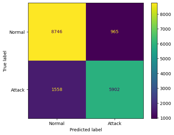
# Making the Confusion Matrix
# [TN, FP ]
# [FN, TP ]
from sklearn.metrics import confusion_matrix, ConfusionMatrixDisplay
cm = confusion_matrix(y_test, y_pred)
print('Print the Confusion Matrix:')
print('[ TN, FP ]')
print('[ FN, TP ]=')
print(cm)
print(classification_report(y_test, y_pred))
disp = ConfusionMatrixDisplay(confusion_matrix=cm, display_labels=['Normal', 'Attack'])
disp.plot()
plt.savefig('confusion_matrix_SB.png')
plt.show()
Print the Confusion Matrix:
[ TN, FP ]
[ FN, TP ]=
[[8746 965]
[1558 5902]]
precision recall f1-score support
0 0.85 0.90 0.87 9711
1 0.86 0.79 0.82 7460
accuracy 0.85 17171
macro avg 0.85 0.85 0.85 17171
weighted avg 0.85 0.85 0.85 17171
Part 4 - Visualizing
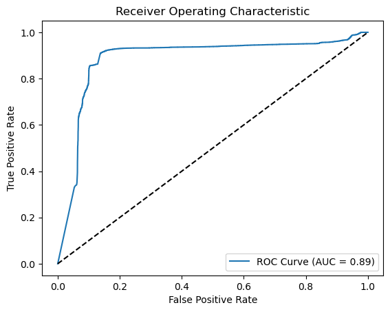
Receiver Operating Characteristic (ROC) Curve and Area Under Curve (AUC)
from sklearn.metrics import roc_curve, auc
import matplotlib.pyplot as plt

# Generate probabilities
y_pred_prob = classifier.predict(X_test).ravel()

# Calculate ROC curve
fpr, tpr, thresholds = roc_curve(y_test, y_pred_prob)
roc_auc = auc(fpr, tpr)

# Plot ROC curve
plt.figure()
plt.plot(fpr, tpr, label=f'ROC Curve (AUC = {roc_auc:.2f})')
plt.plot([0, 1], [0, 1], 'k--')  # Random guess line
plt.xlabel('False Positive Rate')
plt.ylabel('True Positive Rate')
plt.title('Receiver Operating Characteristic')
plt.legend(loc='lower right')
plt.savefig('ROC_SB.png')
plt.show()
537/537 ━━━━━━━━━━━━━━━━━━━━ 19s 35ms/step
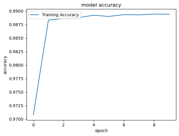
Plot the accuracy
########################################
# Part 4 - Visualizing
#######################################

# Import matplot lib libraries for plotting the figures.
import matplotlib.pyplot as plt

# You can plot the accuracy
print('Plot the accuracy')
# Keras 2.2.4 recognizes 'acc' and 2.3.1 recognizes 'accuracy'
# use the command python -c 'import keras; print(keras.__version__)' on MAC or Linux to check Keras' version
#plt.plot(classifierHistory.history['accuracy'], label='Training Accuracy')
plt.plot(classifierHistory['accuracy'], label='Training Accuracy')
plt.title('model accuracy')
plt.ylabel('accuracy')
plt.xlabel('epoch')
plt.legend(loc='upper left')
plt.savefig('accuracy_sample_SB.png')
plt.show()
Plot the accuracy
Plot the Loss
# You can plot history for loss
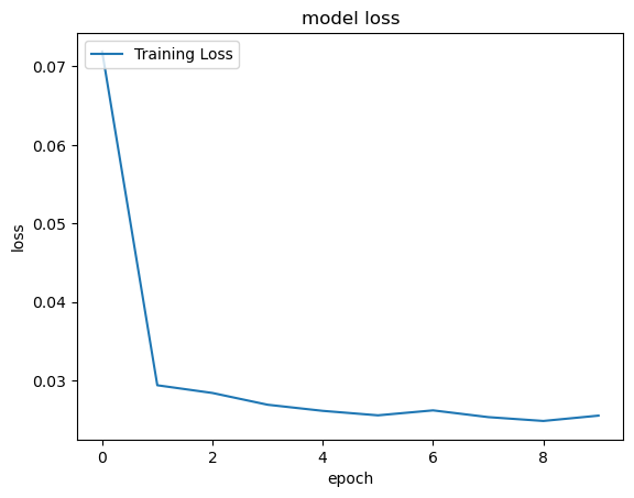
print('Plot the loss')
#plt.plot(classifierHistory.history['loss'], label='Training Loss')
plt.plot(classifierHistory['loss'], label='Training Loss')
plt.title('model loss')
plt.ylabel('loss')
plt.xlabel('epoch')
plt.legend(loc='upper left')
plt.savefig('loss_sample_SB.png')
plt.show()Plot the loss