Section: Ball Throw#
Adapted from: gjbex/Fortran-MOOC
This program demonstrates using the Runge-Kutta method to solve a second order differential equation. The equations of motion for a ball are analyzed.
Runge-Kutta Method Explanation by ChatGPT 4o#
Let’s break down the physical equations governing the motion of the ball, how they are discretized using the Runge-Kutta 4th order (RK4) method, and how the motion of the ball is simulated step-by-step in the code.
1. Physical Model (Equations of Motion)#
The ball is subject to gravity, and we are solving for its trajectory. This can be modeled by the following system of ordinary differential equations (ODEs):
State Variables:#
Position in x: \( X(t) \)
Position in y: \( Y(t) \)
Velocity in x: \( V_X(t) \)
Velocity in y: \( V_Y(t) \)
Equations of Motion:#
The motion of the ball is governed by Newton’s laws of motion. The system of equations is:
Velocity equations (derivatives of position): $\( \frac{dX}{dt} = V_X(t) \)\( \)\( \frac{dY}{dt} = V_Y(t) \)$
Acceleration equations (derivatives of velocity): $\( \frac{dV_X}{dt} = 0 \quad (\text{No horizontal acceleration due to air resistance}) \)\( \)\( \frac{dV_Y}{dt} = -g = -9.81 \, \text{m/s}^2 \quad (\text{Acceleration due to gravity}) \)$
So the full system of ODEs can be written as:
Where:
\( X(t) \) and \( Y(t) \) are the positions in the horizontal and vertical directions.
\( V_X(t) \) and \( V_Y(t) \) are the velocities in the horizontal and vertical directions.
\( g = 9.81 \, \text{m/s}^2 \) is the acceleration due to gravity.
2. Discretization of the Equations Using the Runge-Kutta Method#
The Runge-Kutta 4th order method (RK4) is a numerical method for solving ordinary differential equations. It approximates the solution by calculating intermediate values of the derivatives at multiple points within a time step and combining them to achieve a higher-order approximation.
The system of ODEs can be written as:
Where \( \mathbf{u}(t) \) is the vector of state variables, \( \mathbf{u}(t) = \begin{bmatrix} X(t) \\ Y(t) \\ V_X(t) \\ V_Y(t) \end{bmatrix} \), and \( \mathbf{f}(t, \mathbf{u}) \) is the f function, which is computed by the f subroutine.
In your program, the equations of motion are:
Step 1: The Runge-Kutta Method#
The RK4 method computes the next state vector \( \mathbf{u}(t + \Delta t) \) by evaluating the derivatives at four points within the time step \( \Delta t \) and then combining them. Here’s the mathematical formulation:
Let \( t_0 \) be the current time, and \( \mathbf{u}_0 \) be the current state vector. The Runge-Kutta 4th order method computes the next state \( \mathbf{u}_1 \) at \( t_0 + \Delta t \) as:
The new state vector \( \mathbf{u}_1 \) is given by a weighted sum of these intermediate values:
This formula combines the values at four points: the beginning of the step, the midpoint (evaluated twice), and the end of the step.
Step 2: Applying the RK4 Method to Your System#
Now, let’s apply the RK4 method to your system of equations.
The state vector is:
The RHS function is:
We need to calculate the four approximations ( \( k_1 \), \( k_2 \), \( k_3 \), and \( k_4 \) ) for each of the state variables:
At the current state \( t_0 \), \( \mathbf{u}_0 \):
\[\begin{split} k_1 = \Delta t \, \begin{bmatrix} V_X \\ V_Y \\ 0 \\ -g \end{bmatrix} \end{split}\]At the midpoint \( t_0 + \frac{\Delta t}{2} \), using \( k_1 \) to update \( \mathbf{u}_0 \):
\[\begin{split} k_2 = \Delta t \, \begin{bmatrix} V_X + \frac{k_1(3)}{2} \\ V_Y + \frac{k_1(4)}{2} \\ 0 \\ -g \end{bmatrix} \end{split}\]At the midpoint again, \( t_0 + \frac{\Delta t}{2} \), using \( k_2 \) to update \( \mathbf{u}_0 \):
\[\begin{split} k_3 = \Delta t \, \begin{bmatrix} V_X + \frac{k_2(3)}{2} \\ V_Y + \frac{k_2(4)}{2} \\ 0 \\ -g \end{bmatrix} \end{split}\]At the end of the step \( t_0 + \Delta t \), using \( k_3 \) to update \( \mathbf{u}_0 \):
\[\begin{split} k_4 = \Delta t \, \begin{bmatrix} V_X + k_3(3) \\ V_Y + k_3(4) \\ 0 \\ -g \end{bmatrix} \end{split}\]
Final Update:#
Finally, the updated state \( \mathbf{u}_1 \) is calculated as:
For each component (X, Y, \( V_X \), \( V_Y \)), you apply this formula, updating the state vector by adding the weighted sum of the intermediate steps.
3. Discretization of the Motion#
X and Y (Position):#
For position \( X \), the derivative is \( \frac{dX}{dt} = V_X \).
For position \( Y \), the derivative is \( \frac{dY}{dt} = V_Y \).
At each step, the velocities \( V_X \) and \( V_Y \) are updated, so the positions \( X \) and \( Y \) are updated based on the velocities.
\( V_X \) (Velocity in x-direction):#
The velocity in the x-direction \( V_X \) remains constant (no acceleration in the x-direction):
\[ \frac{dV_X}{dt} = 0 \]This means that \( V_X \) doesn’t change during the simulation.
\( V_Y \) (Velocity in y-direction):#
The velocity in the y-direction is affected by gravity:
\[ \frac{dV_Y}{dt} = -g \]The velocity \( V_Y \) decreases over time due to the downward acceleration caused by gravity.
Summary of the Process#
The ODE system describes the motion of the ball in both the horizontal and vertical directions, with the velocities and positions evolving over time.
The RK4 method discretizes these continuous equations into small steps of size \( \Delta t \). For each step, the
Runge-Kutta method computes intermediate derivatives and combines them to provide an accurate approximation of the solution at the next time step. 3. The results provide the trajectory of the ball, showing how its position and velocity change over time, under the influence of gravity.
This process gives a numerically computed trajectory of the ball thrown at an initial velocity, providing insight into its motion and behavior as time progresses.
Code Analysis by ChatGPT 4o#
Let’s break down the Fortran code in great detail. The program simulates the motion of a ball under the influence of gravity using the fourth-order Runge-Kutta (RK4) method for solving ordinary differential equations (ODEs). Here’s a detailed explanation of each module and subroutine:
1. Main Program: ball_throw#
This is the top-level program that integrates the motion of a ball thrown with initial velocity using RK4.
program ball_throw
    use, intrinsic :: iso_fortran_env, only : DP => real64, int32
    use :: f_mod, only : f
    use :: rk4_mod, only  : rk4vec
    use :: vector_indices_mod, only : X_IDX, Y_IDX, VX_IDX, VY_IDX
    implicit none
    integer, parameter :: NR_EQS = 4
    integer, parameter :: MAX_STEPS = 10000
    real(kind=DP), parameter :: DELTA_T = 0.01_DP
    real(kind=DP) :: t
    real(kind=DP), dimension(NR_EQS) :: u, u_new
    integer :: step
Imports:
iso_fortran_envprovidesreal64(double precision) andint32(32-bit integer) types to ensure consistency in floating-point and integer precision.f_modimports the functionf, which represents the differential equations governing the ball’s motion.rk4_modimports the subroutinerk4vec, which will perform the RK4 integration.vector_indices_modprovides the indices for the state vector components:X_IDX,Y_IDX,VX_IDX, andVY_IDX.
Parameters:
NR_EQS: The number of equations (4, corresponding to position and velocity in both x and y directions).MAX_STEPS: The maximum number of integration steps.DELTA_T: The time step for the RK4 integration (0.01 seconds).
State Vector (
u):This vector holds the state variables: position in
xandy(X_IDX,Y_IDX), and velocity inxandy(VX_IDX,VY_IDX).
Initial Setup:
stepis the step counter.The initial conditions for the ball are set:
u(X_IDX) = 0.0_DP: The initialxposition is 0.u(Y_IDX) = 0.0_DP: The initialyposition is 0.u(VX_IDX) = 5.0_DP: The initial velocity in thexdirection is 5 m/s.u(VY_IDX) = 5.0_DP: The initial velocity in theydirection is 5 m/s.
2. Main Loop:#
    step = 0
    t = 0.0_DP
    u(X_IDX) = 0.0_DP
    u(Y_IDX) = 0.0_DP
    u(VX_IDX) = 5.0_DP
    u(VY_IDX) = 5.0_DP
    print *, step, t, u(X_IDX), u(Y_IDX), u(VX_IDX), u(VY_IDX)

    do step = 1, MAX_STEPS
        call rk4vec(t, NR_EQS, u, DELTA_T, f, u_new)
        t = t + DELTA_T
        u = u_new
        if (u(Y_IDX) < 0.0_DP) exit
        print *, step, t, u(X_IDX), u(Y_IDX), u(VX_IDX), u(VY_IDX)
    end do
Initial Print: The initial values are printed out, showing the time
t, thestep, and the state vector components (x,y,vx,vy).Integration Loop:
The loop runs from
step = 1toMAX_STEPS, performing the RK4 integration for each time step.rk4vecis called to integrate the state vectorufor one step, updating the values inu_new.The time
tis incremented by the step sizeDELTA_T.The state vector
uis updated with the new values fromu_new.The loop exits if the ball’s
yposition (u(Y_IDX)) becomes negative, indicating it has hit the ground.After each step, the current time and state vector are printed.
3. Module: vector_indices_mod#
module vector_indices_mod
    implicit none
    private
    public :: X_IDX, Y_IDX, VX_IDX, VY_IDX
    integer, parameter :: X_IDX = 1
    integer, parameter :: Y_IDX = 2
    integer, parameter :: VX_IDX = 3
    integer, parameter :: VY_IDX = 4
end module vector_indices_mod
This module defines constants representing the indices of the components of the state vector (
u):X_IDX = 1: The index for thexposition.Y_IDX = 2: The index for theyposition.VX_IDX = 3: The index for thexvelocity.VY_IDX = 4: The index for theyvelocity.
4. Module: f_mod#
module f_mod
    use, intrinsic :: iso_fortran_env, only : DP => real64, int32
    use :: vector_indices_mod, only : X_IDX, Y_IDX, VX_IDX, VY_IDX
    implicit none
    private
    public :: f

contains

    subroutine f(t, m, u, uprime)
        implicit none
        real(kind=DP), intent(in) :: t ! Time
        integer(kind=int32), intent(in) :: m ! Number of equations
        real(kind=DP), dimension(m), intent(in) :: u ! State vector
        real(kind=DP), dimension(m), intent(out) :: uprime ! Derivative of the state vector

        real(kind=DP) :: X, Y, VX, VY
        X  = u(X_IDX)   ! Position in x
        Y  = u(Y_IDX)   ! Position in y
        VX = u(VX_IDX)  ! Velocity in x
        VY = u(VY_IDX)  ! Velocity in y

        uprime(X_IDX)  = VX        ! dx/dt = velocity in x
        uprime(Y_IDX)  = VY        ! dy/dt = velocity in y
        uprime(VX_IDX) = 0.0_DP    ! No acceleration in x (ignoring air resistance)
        uprime(VY_IDX) = -9.81_DP  ! Acceleration in y due to gravity
    end subroutine f
end module f_mod
The subroutine
f:This computes the right-hand side of the differential equations, i.e., the derivatives of the state variables.
It takes the current time
t, the number of equationsm, the current state vectoru, and outputs the derivative of the state vectoruprime.State variables:
X,Y: Position inxandy.VX,VY: Velocity inxandy.
Derivatives:
dX/dt = VX: The change inxposition is thexvelocity.dY/dt = VY: The change inyposition is theyvelocity.dVX/dt = 0: There is no acceleration inx(no air resistance).dVY/dt = -9.81: The acceleration inyis due to gravity (constant value -9.81 m/s²).
5. Module: rk4_mod#
This module implements the Runge-Kutta method to integrate the system of ODEs.
subroutine rk4vec ( t0, m, u0, dt, f, u )
    implicit none
    real ( kind = DP ), intent(in) :: t0
    integer ( kind = int32 ), intent(in) :: m
    real ( kind = DP ), dimension(m), intent(in) :: u0
    real ( kind = DP ), intent(in) :: dt
    real ( kind = DP ), dimension(m), intent(out) :: u

    real ( kind = DP ), dimension(m) :: f0, f1, f2, f3
    real ( kind = DP ), dimension(m) :: u1, u2, u3
    real ( kind = DP ) :: t1, t2, t3

    ! Get derivative estimates
    call f ( t0, m, u0, f0 )
    t1 = t0 + dt / 2.0_DP
    u1 = u0 + dt * f0 / 2.0_DP
    call f ( t1, m, u1, f1 )
    t2 = t0 + dt / 2.0_DP


    u2 = u0 + dt * f1 / 2.0_DP
    call f ( t2, m, u2, f2 )
    t3 = t0 + dt
    u3 = u0 + dt * f2
    call f ( t3, m, u3, f3 )

    ! Combine the estimates to compute the next state vector
    u = u0 + ( dt / 6.0_DP ) * ( f0 + 2.0_DP * f1 + 2.0_DP * f2 + f3 )
end subroutine rk4vec
RK4 Method:
The method computes the state vector at the next time step using a weighted average of four intermediate estimates (
f0,f1,f2,f3), corresponding to evaluations of the differential equation at different time points.It allocates arrays for the intermediate state vectors (
u1,u2,u3) and derivative estimates (f0,f1,f2,f3).After computing these estimates using the function
f, the final state vectoruis updated using the formula: $\( u_{t+dt} = u_0 + \frac{dt}{6} \left( f_0 + 2f_1 + 2f_2 + f_3 \right) \)$
Conclusion:#
This program simulates the trajectory of a ball in 2D under gravity. The motion is modeled using 4 first-order ODEs (2 for position, 2 for velocity), which are numerically integrated using the 4th-order Runge-Kutta method. The state vector contains the ball’s position and velocity, and the program outputs the position and velocity at each time step until the ball hits the ground (u(Y_IDX) < 0).
Program Code#
section_ball_throw.f90#
program ball_throw
    use, intrinsic :: iso_fortran_env, only : DP => real64, int32
    use :: f_mod, only : f
    use :: rk4_mod, only  : rk4vec
    use :: vector_indices_mod, only : X_IDX, Y_IDX, VX_IDX, VY_IDX
    implicit none
    integer, parameter :: NR_EQS = 4
    integer, parameter :: MAX_STEPS = 10000
    real(kind=DP), parameter :: DELTA_T = 0.01_DP
    real(kind=DP) :: t
    real(kind=DP), dimension(NR_EQS) :: u, u_new
    integer :: step

    step = 0
    t = 0.0_DP
    u(X_IDX) = 0.0_DP
    u(Y_IDX) = 0.0_DP
    u(VX_IDX) = 5.0_DP
    u(VY_IDX) = 5.0_DP
    print *, step, t, u(X_IDX), u(Y_IDX), u(VX_IDX), u(VY_IDX)

    do step = 1, MAX_STEPS
        call rk4vec(t, NR_EQS, u, DELTA_T, f, u_new)
        t = t + DELTA_T
        u = u_new
        if (u(Y_IDX) < 0.0_DP) exit
        print *, step, t, u(X_IDX), u(Y_IDX), u(VX_IDX), u(VY_IDX)
    end do

end program ball_throw
f_mod.f90#
module f_mod
    use, intrinsic :: iso_fortran_env, only : DP => real64, int32
    use :: vector_indices_mod, only : X_IDX, Y_IDX, VX_IDX, VY_IDX
    implicit none

    private
    public :: f

    contains

        !*******************************************************************************
        subroutine f(t, m, u, uprime)
            implicit none
            real(kind=DP), intent(in) :: t ! Time
            integer(kind=int32), intent(in) :: m ! Number of equations
            real(kind=DP), dimension(m), intent(in) :: u ! State vector
            real(kind=DP), dimension(m), intent(out) :: uprime ! Derivative of the state vector

            ! Declare local variables for the components of the state vector
            real(kind=DP) :: X, Y, VX, VY

            ! Extract state vector components
            X  = u(X_IDX)   ! Position in the x-direction
            Y  = u(Y_IDX)   ! Position in the y-direction
            VX = u(VX_IDX)  ! Velocity in the x-direction
            VY = u(VY_IDX)  ! Velocity in the y-direction

            ! Compute the derivatives (primes)
            uprime(X_IDX)  = VX        ! Derivative of position in x is velocity in x
            uprime(Y_IDX)  = VY        ! Derivative of position in y is velocity in y
            uprime(VX_IDX) = 0.0_DP    ! No acceleration in x (ignoring air resistance)
            uprime(VY_IDX) = -9.81_DP  ! Acceleration in y due to gravity

        end subroutine f
        !*******************************************************************************

end module f_mod
rk4.f90#
module rk4_mod
    use, intrinsic :: iso_fortran_env, only : DP => real64, int32
    use :: f_mod, only : f

    implicit none

    public :: rk4, rk4vec

contains

  !*******************************************************************************
  subroutine rk4 ( t0, u0, dt, u )
  !*******************************************************************************
  !
  !! RK4 takes one Runge-Kutta step for a scalar ODE.
  !
  !  Discussion:
  !
  !    It is assumed that an initial value problem, of the form
  !
  !      du/dt = f ( t, u )
  !      u(t0) = u0
  !
  !    is being solved.
  !
  !    If the user can supply current values of t, u, a stepsize dt, and a
  !    function to evaluate the derivative, this function can compute the
  !    fourth-order Runge Kutta estimate to the solution at time t+dt.
  !
  !  Licensing:
  !
  !    This code is distributed under the GNU LGPL license.
  !
  !  Modified:
  !
  !    31 January 2012
  !    19 December 2024
  !
  !  Author(s):
  !
  !    John Burkardt
  !    Modified by Mark Khusid with ChatGPT 4o (OpenAI)
  !
  !  Parameters:
  !
  !    Input, real ( kind = 8 ) T0, the current time.
  !
  !    Input, real ( kind = 8 ) U0, the solution estimate at the current time.
  !
  !    Input, real ( kind = 8 ) DT, the time step.
  !
  !    Input, external F, a subroutine of the form
  !      subroutine f ( t, u, uprime )
  !    which evaluates the derivative uprime given the time T and
  !    solution vector U.
  !
  !    Output, real ( kind = 8 ) U, the fourth-order Runge-Kutta solution
  !    estimate at time T0+DT.
  !
    implicit none

    ! Current time
    real ( kind = DP ), intent(in) :: t0

    ! Initial state vector at time t0
    real ( kind = DP ), dimension(:), intent(in) :: u0

    ! Time step
    real ( kind = DP ), intent(in) :: dt

    ! Output argument: updated state vector at time t0 + dt
    real ( kind = DP ), dimension(:), intent(out) :: u

    ! Local variables

    integer :: m

    ! Derivative estimates at different stages of the Runge-Kutta method
    real ( kind = DP ), dimension(:), allocatable :: f0, f1, f2, f3

    ! Intermediate state vectors at different stages of the Runge-Kutta method
    real ( kind = DP ), dimension(:), allocatable :: u1, u2, u3

    ! Intermediate times at different stages of the Runge-Kutta method
    real ( kind = DP ) :: t1, t2, t3

    ! Get the size of the state vector
    m = size(u0)

    ! Allocate memory for the derivative estimates and intermediate state vectors
    allocate(f0(m), f1(m), f2(m), f3(m))
    allocate(u1(m), u2(m), u3(m))

    ! Step 1: Evaluate the derivative at the initial time and state
    call f ( t0, m, u0, f0 )

    ! Step 2: Compute the intermediate state and derivative at the midpoint 1 of the interval
    t1 = t0 + dt / 2.0_DP
    u1 = u0 + dt * f0 / 2.0_DP
    call f ( t1, m, u1, f1 )

    ! Step 3: Compute the intermediate state and derivative at the midpoint 2 of the interval
    t2 = t0 + dt / 2.0_DP
    u2 = u0 + dt * f1 / 2.0_DP
    call f ( t2, m, u2, f2 )

    ! Step 4: Compute the intermediate state and derivative at the end of the interval
    t3 = t0 + dt
    u3 = u0 + dt * f2
    call f ( t3, m, u3, f3 )

    ! Step 5: Combine the four estimates to update the solution at t0 + dt
    u = u0 + (dt / 6.0_DP) * ( f0 + 2.0_DP * f1 + 2.0_DP * f2 + f3 )

    ! Deallocate the temporary arrays
    deallocate(f0, f1, f2, f3)
    deallocate(u1, u2, u3)

  end subroutine rk4
  !*******************************************************************************

  !*******************************************************************************
  subroutine rk4vec ( t0, m, u0, dt, f, u )
  !*****************************************************************************80
  !
  !! RK4VEC takes one Runge-Kutta step for a vector ODE.
  !
  !  Discussion:
  !
  !    Thanks to Dante Bolatti for correcting the final function call to:
  !      call f ( t3, m, u3, f3 )
  !    18 August 2016.
  !
  !  Licensing:
  !
  !    This code is distributed under the GNU LGPL license.
  !
  !  Modified:
  !
  !    18 August 2016
  !    19 December 2024
  !
  !  Author(s):
  !
  !    John Burkardt
  !    Modified by Mark Khusid with ChatGPT 4o (OpenAI)
  !
  !  Parameters:
  !
  !    Input, real ( kind = 8 ) T0, the current time.
  !
  !    Input, integer ( kind = 4 ) M, the dimension of the system.
  !
  !    Input, real ( kind = 8 ) U0(M), the solution estimate at the current time.
  !
  !    Input, real ( kind = 8 ) DT, the time step.
  !
  !    Input, external F, a subroutine of the form
  !      subroutine f ( t, m, u, uprime )
  !    which evaluates the derivative UPRIME(1:M) given the time T and
  !    solution vector U(1:M).
  !
  !    Output, real ( kind = 8 ) U(M), the fourth-order Runge-Kutta solution
  !    estimate at time T0+DT.
  !
    implicit none

    interface
      subroutine f ( t, m, u, uprime )
        use, intrinsic :: iso_fortran_env, only : DP => real64, int32
        real ( kind = DP ), intent(in) :: t
        integer ( kind = int32 ), intent(in) :: m
        real ( kind = DP ), dimension(m), intent(in) :: u
        real ( kind = DP ), dimension(m), intent(out) :: uprime
      end subroutine f
    end interface

    ! Input arguments
    ! Current time
    real ( kind = DP ), intent(in) :: t0

    ! Dimension of the system
    integer ( kind = int32 ), intent(in) :: m

    ! Initial state vector at time t0
    real ( kind = DP ), dimension(m), intent(in) :: u0

    ! Time step
    real ( kind = DP ), intent(in) :: dt

    ! Output argument: updated state vector at time t0 + dt
    real ( kind = DP ), dimension(m), intent(out) :: u

    ! Local variables
    ! Derivative estimates at different stages of the Runge-Kutta method
    real ( kind = DP ), dimension(m) :: f0, f1, f2, f3

    ! Intermediate state vectors at different stages of the Runge-Kutta method
    real ( kind = DP ), dimension(m) :: u1, u2, u3

    ! Intermediate times at different stages of the Runge-Kutta method
    real ( kind = DP ) :: t1, t2, t3

  !  Get four sample values of the derivative.
    ! Step 1: Evaluate the derivative at the initial time and state
    call f ( t0, m, u0, f0 )

    ! Step 2: Compute the intermediate state and derivative at the midpoint 1 of the interval
    t1 = t0 + dt / 2.0_DP
    u1 = u0 + dt * f0 / 2.0_DP
    call f ( t1, m, u1, f1 )

    ! Step 3: Compute the intermediate state and derivative at the midpoint 2 of the interval
    t2 = t0 + dt / 2.0_DP
    u2 = u0 + dt * f1 / 2.0_DP
    call f ( t2, m, u2, f2 )

    ! Step 4: Compute the intermediate state and derivative at the end of the interval
    t3 = t0 + dt
    u3 = u0 + dt * f2
    call f ( t3, m, u3, f3 )
  !
  !  Combine them to estimate the solution U at time T1.
  ! Step 5: Combine the four estimates to update the solution at t0 + dt
    u = u0 + ( dt / 6.0_DP ) * ( f0 + 2.0_DP * f1 + 2.0_DP * f2 + f3 )

  end subroutine rk4vec
  !*******************************************************************************

end module rk4_mod
vector_indices_mod.f90#
module vector_indices_mod
    ! This module defines the indices for the state vector components
    implicit none

    private

    public :: X_IDX, Y_IDX, VX_IDX, VY_IDX

    integer, parameter :: X_IDX = 1
    integer, parameter :: Y_IDX = 2
    integer, parameter :: VX_IDX = 3
    integer, parameter :: VY_IDX = 4

end module vector_indices_mod
The above program is compiled and run using Fortran Package Manager (fpm). The following FPM configuration file (fpm.toml) was used:
name = "Section_Ball_Throw"

[build]
auto-executables = true
auto-tests = true
auto-examples = true

[install]
library = false

[[executable]]
name="Section_Ball_Throw"
source-dir="app"
main="section_ball_throw.f90"
Build the Program using FPM (Fortran Package Manager)#
import os
root_dir = ""
root_dir = os.getcwd()
code_dir = root_dir + "/" + "Fortran_Code/Section_Ball_Throw"
os.chdir(code_dir)
build_status = os.system("fpm build 2>/dev/null")
Run the Program using FPM (Fortran Package Manager)#
The program is run and the output is saved into a file named ‘data.dat
exec_status = \
    os.system("fpm run > data.dat 2>/dev/null")
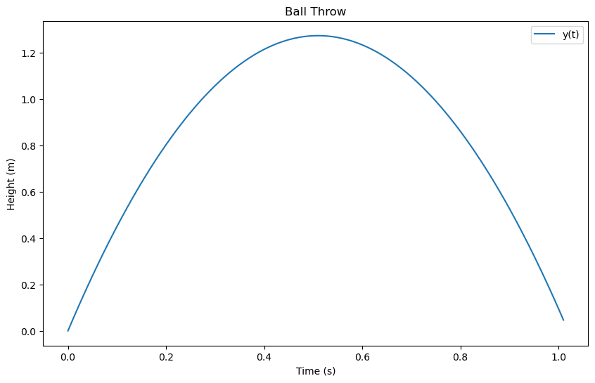
Plot the Trajectory of the Ball#
%matplotlib inline
import matplotlib.pyplot as plt
import numpy as np
data = np.loadtxt("data.dat")
time = [row[1] for row in data]
y    = [row[3] for row in data]
fig, ax = plt.subplots(figsize=(10, 6))
ax.plot(time, y, label='y(t)')
ax.set_xlabel('Time (s)')
ax.set_ylabel('Height (m)')
ax.set_title('Ball Throw')
ax.legend()
plt.show()