Discretized Fourier Transform of Arbitrary Signal Using FFTW3 in Fortran

Table of Contents

• Sine Wave at 10Hz
• Square Wave at 1Hz
• Two Sine Waves with Different Frequencies
• Switched 1 kHz Sine Wave

Introduction

The Discrete Fourier Transform (DFT) is a mathematical technique used to convert a signal from its time domain representation to its frequency domain representation. The DFT is defined as follows:

\[ X(k) = \sum_{n=0}^{N-1} x(n) e^{-j2\pi kn/N} \]

where \(X(k)\) is the DFT of the signal \(x(n)\), \(N\) is the number of samples in the signal, and \(k\) is the frequency index. The DFT is a powerful tool in signal processing and is used in a wide range of applications, including audio and image processing, communications, and control systems.

The Fast Fourier Transform (FFT) is an algorithm that computes the DFT of a signal more efficiently than the standard DFT algorithm. The FFT algorithm exploits the symmetry properties of the DFT to reduce the number of computations required to compute the DFT. The FFT algorithm is widely used in practice due to its speed and efficiency.

In this tutorial, we will use the FFTW3 library to compute the DFT of an arbitrary signal. FFTW3 is a highly optimized library for computing the FFT of a signal and is widely used in scientific computing applications. We will demonstrate how to use the FFTW3 library to compute the DFT of a signal and visualize the frequency spectrum of the signal.

Prerequisites

To follow this tutorial, you will need:

• A basic understanding of Fortran programming

• A working Fortran compiler (e.g., gfortran)

• The FFTW3 library installed on your system

Installing FFTW3

The FFTW3 library is a free and open-source library that can be downloaded from the FFTW website. To install FFTW3 on your system, follow these steps:

1. Download the FFTW3 library from the FFTW website.

2. Extract the contents of the downloaded archive to a directory on your system.

3. Run the following commands to configure, compile, and install the FFTW3 library:

./configure
make
make install

Computing the DFT Using FFTW3

To compute the DFT of an arbitrary signal using FFTW3, follow these steps:

1. Include the FFTW3 module in your Fortran program:

use, intrinsic :: iso_c_binding
use fftw3

2. Define the size of the input signal and allocate memory for the input and output arrays:

integer, parameter :: N = 1024
real(c_double), dimension(N) :: x
complex(c_double), dimension(N) :: X

3. Create a plan for computing the FFT of the input signal:

type(c_ptr) :: plan
plan = fftw_plan_dft_1d(N, c_loc(x), c_loc(X), FFTW_FORWARD, FFTW_ESTIMATE)

4. Generate a sample input signal (e.g., a sinusoidal signal) and compute its DFT:

do i = 1, N
    x(i) = sin(2.0 * 3.14159 * i / N)
end do
call fftw_execute_dft(plan, c_loc(x), c_loc(X))

5. Visualize the frequency spectrum of the input signal using a plotting library (e.g., gnuplot):

open(unit=10, file='spectrum.dat', status='unknown')
do i = 1, N
    write(10, *) i, abs(X(i))
end do
close(10)

6. Plot the frequency spectrum using gnuplot:

gnuplot -persist -e "plot 'spectrum.dat' with lines"

Discussion

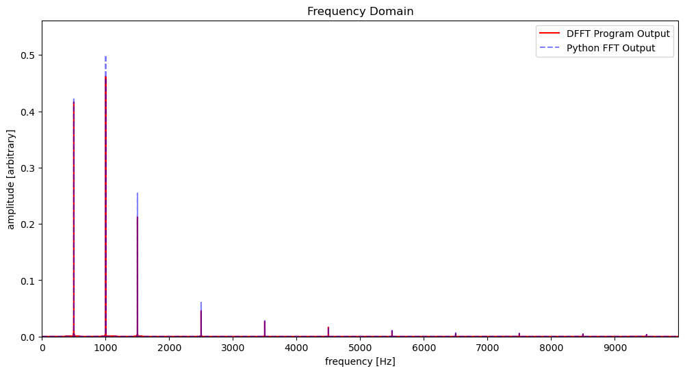
The plan here is to write a Fortran 2003 program that utilizes the FFTW3 library to generate a Discretized Fast Fourier Transforms of arbitrary waveforms. To test the code we start with a function whose DFFT is easily identifiable by inspection, and then increase in complexity. SciLAB and Python+Numpy on Jupyter Notebook are used to generate the the time domain functions, time domain and frequency domain plots and discretized time domain data. The Fortran 2003 code is then run on the discretized time domain data and the results plotted with GNUPlot. A comparison is made to check the veracity of the Fortran 2003 code output.

Examples

The following examples demonstrate the computation of the DFT of an arbitrary signal using the FFTW3 library in Fortran.

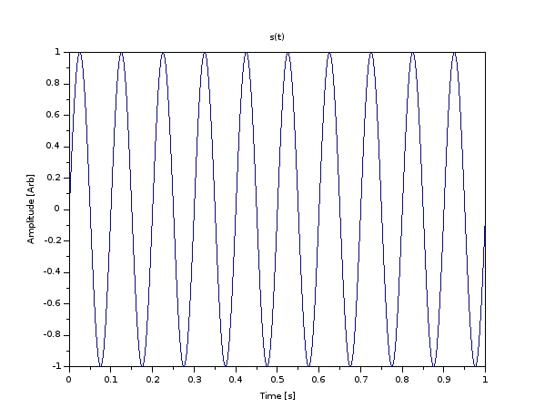
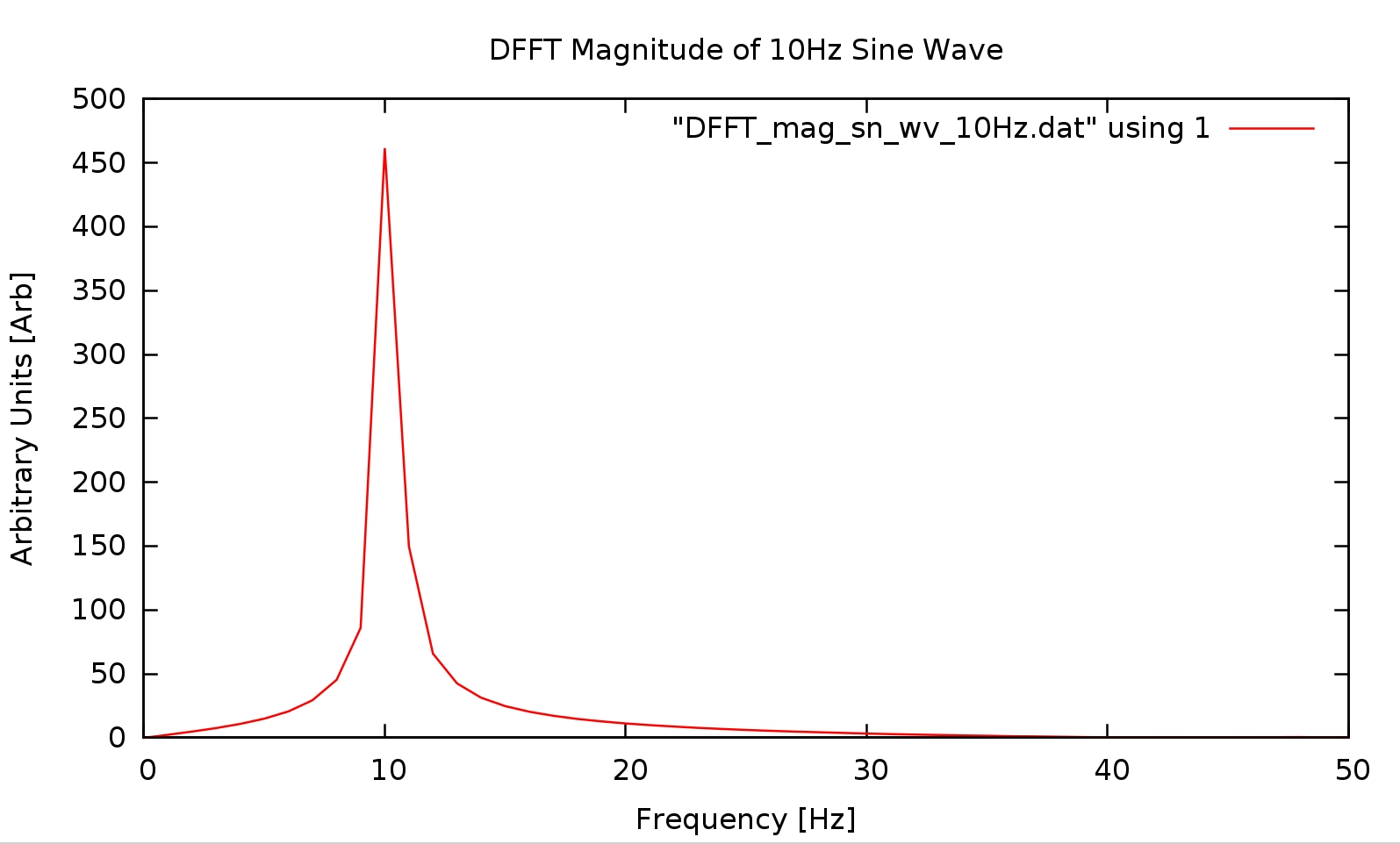
Sine Wave at 10 Hz

Sine_Wave_10_Hz/sine_wave_10_hz.html

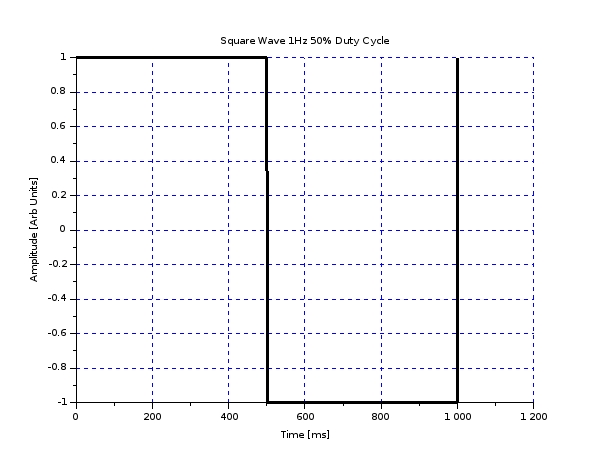
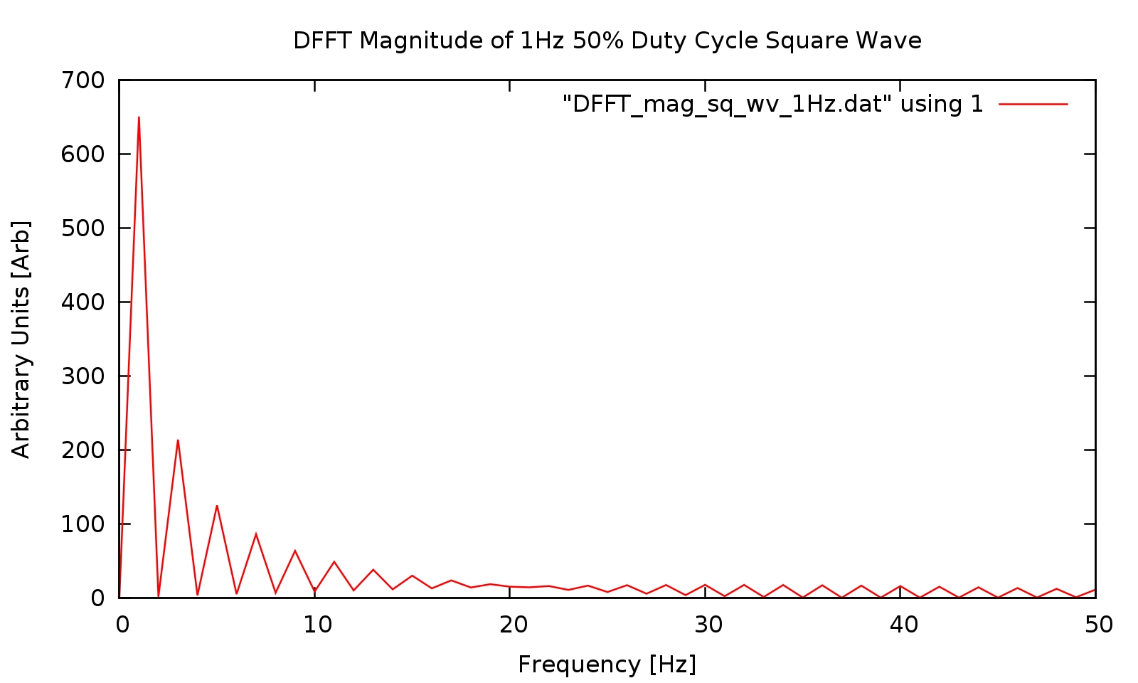
Square Wave at 1 Hz with 50% Duty Cycle

Square_Wave_1_Hz_50_pct/square_wave_1_hz_50_pct.html

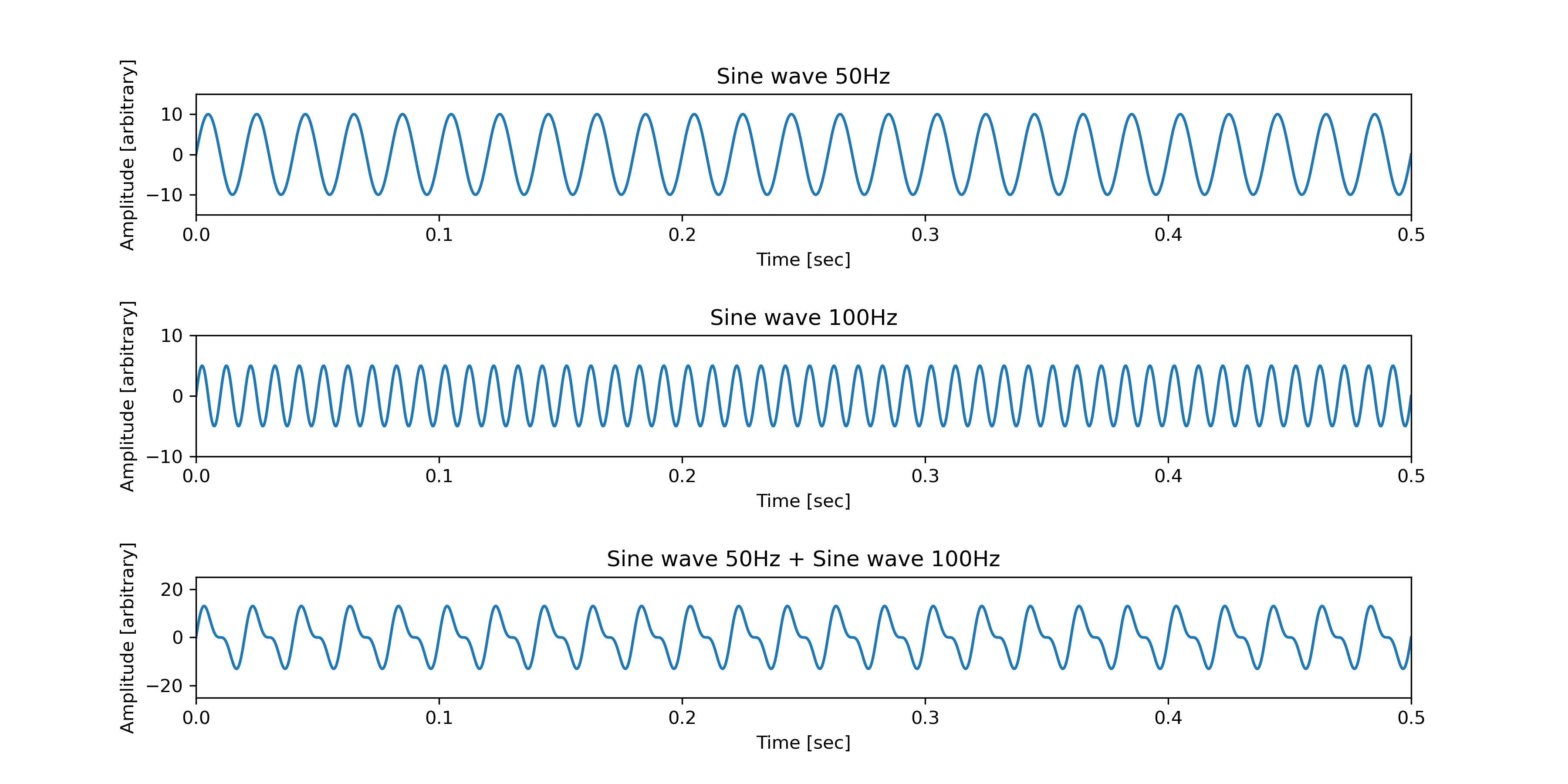
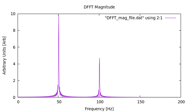
Two Sine Waves at 50 Hz and 100 Hz

2_Sine_Waves/2sineXHz.html

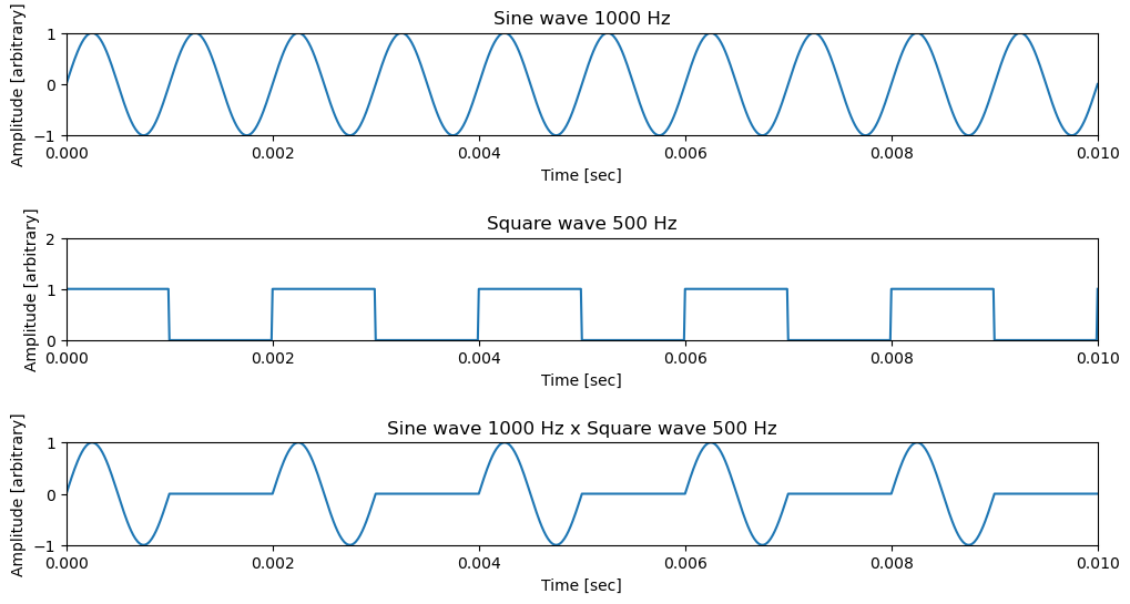
Switched Sine Wave at 1 kHz

Switched_Sine_Wave_1_kHz/switched_sine_wave_1_kHz.html

Conclusion

In this tutorial, we have demonstrated how to compute the Discrete Fourier Transform (DFT) of an arbitrary signal using the FFTW3 library in Fortran. The FFTW3 library provides a fast and efficient way to compute the DFT of a signal and is widely used in scientific computing applications. By following the steps outlined in this tutorial, you can compute the DFT of a signal and visualize its frequency spectrum using the FFTW3 library.