Neural Fortran Examples: Sine Wave

Introduction

In this example, we will train a neural network to approximate the sine function. We will use a simple feedforward neural network with two hidden layers. The network will be trained using the backpropagation algorithm. The data will be written to a CSV file using the CSV Fortran library jacobwilliams/csv-fortran. The neural network will be implemented in Fortran using the Neural Fortran library modern-fortran/neural-fortran.

Once the data is collected and saved to a CSV file, Pandas and Matplotlib will be used to plot the learned sine wave and mean squared error versus the learning iteration number.

Neural Network Theory by ChatGPT o1

Below is a concise yet mathematically grounded overview of dense neural networks, sometimes referred to as feedforward or fully connected networks. We will cover their core structure, forward-pass equations, and typical training approach.

---

Dense Neural Network Structure

A dense (fully connected) neural network consists of layers of neurons, where each neuron in one layer connects to every neuron in the next layer via a trainable weight. Suppose we have a network with \(L\) layers, indexed by \( \ell = 1, 2, \ldots, L\). Each layer \(\ell\) has \(n_\ell\) neurons. For simplicity, let \(\mathbf{x} \in \mathbb{R}^{n_0}\) be the input, where \(n_0\) is the input dimension, and let \(\mathbf{y} \in \mathbb{R}^{n_L}\) be the network’s output.

A typical layer \(\ell\) of the network (for \(1 \le \ell \le L\)) is described by a linear transformation followed by an elementwise non-linear activation. Specifically,

\[ \mathbf{z}^{(\ell)} \;=\; W^{(\ell)}\, \mathbf{h}^{(\ell-1)} \;+\; \mathbf{b}^{(\ell)}, \]

where:

• \(W^{(\ell)} \in \mathbb{R}^{n_\ell \times n_{\ell-1}}\) is the weight matrix for layer \(\ell\).

• \(\mathbf{b}^{(\ell)} \in \mathbb{R}^{n_\ell}\) is the bias vector.

• \(\mathbf{h}^{(\ell-1)} \in \mathbb{R}^{n_{\ell-1}}\) is the output (also called the activation) of the previous layer (\(\ell-1\)).

Next, we apply a (usually nonlinear) activation function \(\sigma(\cdot)\) elementwise:

\[\begin{split} \mathbf{h}^{(\ell)} \;=\; \sigma\bigl(\mathbf{z}^{(\ell)}\bigr) \;=\; \begin{bmatrix} \sigma(z_1^{(\ell)}) \\[6pt] \sigma(z_2^{(\ell)}) \\[6pt] \vdots \\[6pt] \sigma(z_{n_\ell}^{(\ell)}) \\[6pt] \end{bmatrix}. \end{split}\]

For instance, \(\sigma\) might be the ReLU function \(\max(0, z)\), the sigmoid function \(\tfrac{1}{1 + e^{-z}}\), or \(\tanh\). The final output layer might also have a special activation (e.g., softmax for classification).

---

Forward Pass Equations

Using the above notation, we initialize the network’s input as

\[ \mathbf{h}^{(0)} \;=\; \mathbf{x}. \]

Then for each layer \(\ell = 1, 2, \ldots, L\), we compute

\[ \mathbf{z}^{(\ell)} = W^{(\ell)}\, \mathbf{h}^{(\ell-1)} + \mathbf{b}^{(\ell)}, \quad \mathbf{h}^{(\ell)} = \sigma\bigl(\mathbf{z}^{(\ell)}\bigr). \]

At the final layer, \(\mathbf{h}^{(L)}\) becomes the network’s output \(\mathbf{y}\). Hence, a forward pass through a dense network is just iterating these matrix-vector multiplications and elementwise activations.

---

Training With Gradient Descent

To train the network, we typically have a dataset of inputs \(\{\mathbf{x}_i\}\) and corresponding targets \(\{\mathbf{t}_i\}\). We define a loss function \(\mathcal{L}\), such as mean squared error (for regression) or cross-entropy (for classification). For a single training example \((\mathbf{x}, \mathbf{t})\), we might write

\[ \mathcal{L}(\mathbf{t}, \mathbf{y}) \;=\; \frac{1}{2} \|\mathbf{y} - \mathbf{t}\|^2 \quad\text{(for an example squared error case).} \]

The backpropagation algorithm computes partial derivatives of \(\mathcal{L}\) with respect to each network parameter \(\{W^{(\ell)}, \mathbf{b}^{(\ell)}\}\). Gradient-based optimizers (e.g., stochastic gradient descent) then update the parameters in the direction that reduces the loss:

\[ W^{(\ell)} \;\leftarrow\; W^{(\ell)} \;-\; \eta \,\frac{\partial \mathcal{L}}{\partial W^{(\ell)}} \quad,\quad \mathbf{b}^{(\ell)} \;\leftarrow\; \mathbf{b}^{(\ell)} \;-\; \eta \,\frac{\partial \mathcal{L}}{\partial \mathbf{b}^{(\ell)}}, \]

where \(\eta\) is the learning rate. Repeated over many iterations (epochs), the network learns weights that (hopefully) minimize the loss on the training set and generalize to unseen data.

---

This dense architecture is the foundational design for many neural networks. While modern advances (like convolutional or transformer layers) may structure connections differently, the core linear+activation principle remains central to deep learning.

Code Analysis by ChatGTP o1

Below is a detailed walkthrough of how the program sine works, focusing on what each block of code accomplishes and how it fits into the overall workflow of training a sine-wave–inspired neural network. We will cover:

1. Imports and Declarations

2. CSV Logging Initialization

3. Creating Test Data

4. Defining the Neural Network

5. Training Loop (Forward & Backward passes, updating weights)

6. Computing Mean Squared Error

7. Logging Data to CSV

Throughout, note that the network code comes from a library nf (with dense, input, network, sgd), and CSV output is handled by csv_module. The code also uses single-precision real numbers (real32) for training variables and a double-precision pi in some places.

---

1. Imports and Declarations

program sine
  use csv_module
  use nf, only: dense, input, network, sgd
  use iso_fortran_env, only: real32

  implicit none

  real, parameter :: pi = 4 * atan(1.)

1. csv_module: A module that provides CSV reading/writing functionality.

2. nf: A custom or third-party neural network framework that exposes:

   • dense: A fully connected (dense) layer constructor.

   • input: An input layer constructor.

   • network: A type or class that composes layers and provides forward, backward, update, predict.

   • sgd: A function or type for the Stochastic Gradient Descent optimizer.

3. iso_fortran_env, only: real32: Imports the real32 kind for single-precision floats (32-bit).

4. implicit none: Requires explicit declarations for all variables.

5. pi: Defined via 4 * atan(1.), which yields \(\pi \approx 3.14159265...\).

---

2. CSV Logging Initialization

  type(csv_file) :: sine_NN_data_file
  type(network) :: net

  logical :: status_ok

• sine_NN_data_file: A csv_file object that will handle CSV writing.

• net: A neural network object.

  integer, parameter :: num_iterations = 100000
  integer, parameter :: test_size = 50
  real(kind=real32), parameter :: learning_rate = 0.1

• num_iterations: The number of training iterations (epochs).

• test_size: The number of data points for both testing and each training mini-batch (30).

• learning_rate: The initial learning rate (0.1) for the sgd optimizer.

---

3. Neural Network Dimensions and Data Arrays

  integer, parameter :: num_inputs = 1
  integer, parameter :: num_outputs = 1
  integer, parameter :: num_neurons_first_layer = 10
  integer, parameter :: num_neurons_second_layer = 10

• num_inputs: The network expects 1D input.

• num_outputs: The network outputs 1 value.

• num_neurons_first_layer, num_neurons_second_layer: Two hidden layers with 10 neurons each.

  real(kind=real32), dimension(test_size) :: x_test, y_test, x_train, y_train, y_pred
  real, dimension(1) :: x_train_arr_temp
  real, dimension(1) :: y_train_arr_temp
  real, dimension(1) :: x_test_arr_temp
  real, dimension(1) :: y_pred_arr_temp

1. x_test, y_test: Arrays of size test_size to store the input and target for the sine wave test set.

2. x_train, y_train: Arrays of size test_size for the random training mini-batch each iteration.

3. y_pred: Predictions made on the test data, also size test_size.

4. x_train_arr_temp, y_train_arr_temp, x_test_arr_temp, y_pred_arr_temp: All dimension(1).

   • These hold single-sample data for the neural network calls. The library expects arrays, even for single-value input.

   • For instance, x_train(j) is stored in x_train_arr_temp(1) before calling forward.

  real(kind=real32), dimension(num_iterations) :: mean_squared_error
  integer :: i, j

  real(kind=real32) :: x_train_temp

• mean_squared_error: An array storing MSE for each of the num_iterations.

• x_train_temp: A random value used to generate the training data.

---

3.1 CSV File Initialization

  call sine_NN_data_file%initialize(verbose=.true.)
  ...
  call sine_NN_data_file%open('sine_NN_data.csv', n_cols=7, status_ok=status_ok)
  if (.not. status_ok) then
    ...
  end if
  ...
  call sine_NN_data_file%add(['Iteration', 'x_test___', 'y_test___', &
                              'x_train__', 'y_train__', 'y_pred___', 'MSE______'])
  call sine_NN_data_file%next_row()

1. initialize: Prepares the CSV object.

2. open: Opens a file named sine_NN_data.csv. The code also specifies n_cols=7, meaning each row will eventually have up to 7 columns.

3. Header: add([...]) writes a header row with column labels, then next_row() finalizes that line.

---

4. Creating Test Data

  x_test = [((j - 1) * 2.0d0 * pi / test_size, j = 1, test_size)]
  y_test = (sin(x_test) + 1.0d0) / 2.0d0

• For each j in [1..test_size], compute \(\displaystyle x\_test(j) = \frac{(j - 1)\times 2\pi}{\text{test\_size}}\).

  • This distributes 30 points evenly between 0 and 2π.

• The target is y_test(j) = (sin(x_test(j)) + 1) / 2, mapping the sine wave from [-1, +1] to [0, 1].

---

5. Constructing the Neural Network

  net = network([ &
    input(num_inputs), &
    dense(num_neurons_first_layer), &
    dense(num_neurons_second_layer), &
    dense(num_outputs) &
  ])

• network([...]): Creates a layered neural network object with the following sequence:

  1. input(num_inputs): 1D input layer.

  2. dense(num_neurons_first_layer): A fully connected layer with 10 neurons.

  3. dense(num_neurons_second_layer): Another hidden layer with 10 neurons.

  4. dense(num_outputs): Final layer that outputs a single value.

  call net % print_info()

• Prints summary info about the network (number of parameters, layer shapes, etc.).

---

6. Training Loop

  do i = 1, num_iterations

A loop over the total epochs (num_iterations = 100,000). Each iteration does:

6.1 Mini-Batch Data Generation

    do j = 1, test_size
      call random_number(x_train_temp)
      x_train(j) = x_train_temp * 2.0d0 * pi
      y_train(j) = (sin(x_train(j)) + 1.0d0) / 2.0d0

• For each of the test_size samples in the batch:

  1. Generate a random number x_train_temp in [0, 1).

  2. Scale it to [0, 2π].

  3. Compute y_train(j) as (sin(x_train(j)) + 1.0)/2.0, so the sine wave is in [0, 1].

6.2 Per-Sample Forward/Backward

      x_train_arr_temp = x_train(j)
      y_train_arr_temp = y_train(j)

      call net % forward(x_train_arr_temp)
      call net % backward(y_train_arr_temp)
      call net % update(optimizer=sgd(learning_rate=learning_rate))

• x_train_arr_temp and y_train_arr_temp are 1-element arrays. Some neural net frameworks require arrays even for single-value inputs.

• forward(...) passes the single sample through the network, producing internal activations.

• backward(...) uses the single-sample label y_train_arr_temp to compute gradients (loss derivative w.r.t. weights).

• update(...) applies Stochastic Gradient Descent with learning_rate=0.1 to update network weights.

Important: This code does a per-sample update inside the loop over j. This is effectively “online” or “sample-by-sample” training, repeated test_size times per iteration.

6.3 Prediction on the Test Sample

      x_test_arr_temp = x_test(j)
      y_pred_arr_temp = net % predict(x_test_arr_temp)
      y_pred(j) = y_pred_arr_temp(1)
    end do

• Takes the test input x_test(j), passes it through the network to get y_pred_arr_temp (again a 1-element array).

• Store y_pred(j) = y_pred_arr_temp(1).

After this inner loop, we have:

• A mini-batch of test_size random training samples used for weight updates.

• y_pred for each of the 30 test points in x_test.

---

6.4 Compute Mean Squared Error

    mean_squared_error(i) = sum((y_pred - y_test)**2) / test_size

• Compare the network’s predictions y_pred with the true test values y_test.

• The MSE for iteration i is the average of squared differences.

---

6.5 Logging Each Sample to CSV

    do j = 1, test_size
      call sine_NN_data_file%add([i], int_fmt='(i6)')
      call sine_NN_data_file%add([ &
        x_test(j), & 
        y_test(j), &
        x_train(j), &
        y_train(j), &
        y_pred(j), &
        mean_squared_error(i)], &
        real_fmt='(f9.6)')
      call sine_NN_data_file%next_row()
    end do

• We output 50 rows per iteration. Each row records:

  1. Iteration number i.

  2. x_test(j): The j-th test input.

  3. y_test(j): The sine wave’s true value at x_test(j).

  4. x_train(j): The j-th random training sample.

  5. y_train(j): The training label for that sample.

  6. y_pred(j): The network’s prediction for x_test(j).

  7. mean_squared_error(i): The iteration’s MSE.

Hence, each iteration appends 50 lines to the CSV file, for a total of: \(50 \times \text{num_iterations}\) lines.

---

6.6 Occasional Print of MSE

    if (mod(i, (num_iterations/10)) == 0) then
      print '("Iteration: ", I6, " | MSE: ", F9.6)', i, mean_squared_error(i)
    end if

• Every 1/10th of num_iterations (in this case, every 10000 iterations if num_iterations=100000), print the iteration number and current MSE to the console.

---

7. Closing Steps

  print *, '[*] Training complete!'
  print *, '[*] Saving data to the CSV file...'
  ...
  call sine_NN_data_file%close(status_ok=status_ok)
  if (.not. status_ok) then
    print *, '[!] Error closing the CSV file...'
    stop
  end if
end program sine

• Signals the end of training and closes the CSV file, ensuring everything is written to disk properly.

---

8. Summary of the Workflow

1. Initialize: Creates a CSV object, sets up the neural network, and preps hyperparameters.

2. Generate a small, fixed test set (x_test, y_test) spanning 0 to \(2\pi\).

3. Create the network with 1 input neuron, two hidden layers of 10 each, and 1 output.

4. Training (outer loop over i):

   • Build a random mini-batch of test_size samples (x_train, y_train).

   • For each sample:

     • Convert the single value to a 1-element array, do forward/backward/update.

     • Predict on the corresponding test sample x_test(j).

   • Compute MSE over all 50 test points.

   • Write iteration data (50 rows) into a CSV file.

   • Occasionally print progress.

5. Finish: Print completion message, close the CSV file.

Key Observations:

• The code mixes “training data” that’s random each iteration with a fixed “test set” (x_test). This is somewhat unusual—often you keep a consistent training set or you randomize from a larger pool. But it works here as a demonstration of incremental training for the sine function.

• The network is updated on a per-sample basis, repeated 50 times per iteration. That’s effectively a “mini-batch” of size 1 repeated 50 times.

• The final CSV ends up quite large: num_iterations × test_size lines, with 7 columns each.

This design shows how to integrate data generation, single-sample training steps, and CSV logging within a single Fortran program using a custom network library.

Program Code

section_examples_sine_wave.f90

program sine
  use csv_module
  use nf, only: dense, input, network, sgd
  use iso_fortran_env, only: real32

  implicit none

  real, parameter :: pi = 4 * atan(1.)
  
  ! CSV file objects for the training, testing, and prediction data
  type(csv_file) :: sine_NN_data_file
  type(network) :: net

  ! Status of the CSV file operations
  logical :: status_ok
 
  ! Neural Network Training parameters
  integer, parameter :: num_iterations = 100000
  integer, parameter :: test_size = 50
  real(kind=real32), parameter :: learning_rate = 0.1
  
  ! Neural Network (Fully Connected) Parameters
  integer, parameter :: num_inputs = 1
  integer, parameter :: num_outputs = 1
  integer, parameter :: num_neurons_first_layer = 10
  integer, parameter :: num_neurons_second_layer = 10

  ! Training, Testing, and Prediction Data
  real(kind=real32), dimension(test_size) :: x_test, y_test, x_train, y_train, y_pred
  real, dimension(1) :: x_train_arr_temp
  real, dimension(1) :: y_train_arr_temp
  real, dimension(1) :: x_test_arr_temp
  real, dimension(1) :: y_pred_arr_temp
  
  ! Mean Squared Error
  real(kind=real32), dimension(num_iterations) :: mean_squared_error

  ! Loop variables
  integer :: i, j

  ! Temporary variables
  real(kind=real32) :: x_train_temp

  ! Initialize the CSV file
  call sine_NN_data_file%initialize(verbose=.true.)
  
  ! Open the CSV file
  print *, '[*] Opening the CSV file...'
  call sine_NN_data_file%open('sine_NN_data.csv', n_cols=7, status_ok=status_ok)
  if (.not. status_ok) then
    print *, '[!] Error opening the CSV file...'
    stop
  end if

  ! Add header to the CSV file
  print *, '[*] Adding header to the CSV file...'
  call sine_NN_data_file%add(['Iteration', 'x_test___', 'y_test___', 'x_train__', 'y_train__', 'y_pred___', 'MSE______'])
  call sine_NN_data_file%next_row()
  
  print '("[*] Creating Sine Wave Testing Data")'

  ! Create the Sine Wave Testing Data
  x_test = [((j - 1) * 2.0d0 * pi / test_size, j = 1, test_size)]
  y_test = (sin(x_test) + 1.0d0) / 2.0d0

  ! Create the Neural Network
  print *, '[*] Creating the Neural Network...'
  print '(60("="))'
  net = network([ &
    input(num_inputs), &
    dense(num_neurons_first_layer), &
    dense(num_neurons_second_layer), &
    dense(num_outputs) &
  ])

  ! Print the Neural Network information
  call net % print_info()
  print *

  ! Train the Neural Network
  print *, '[*] Training the Neural Network...'
  print '(60("="))'

  ! Loop over the number of iterations (epochs)
  do i = 1, num_iterations

    ! Train the Neural Network on the mini - batch of training data
    do j = 1, test_size
      ! Generate a random mini - batch of training data
      call random_number(x_train_temp)
      x_train(j) = x_train_temp * 2.0d0 * pi
      y_train(j) = (sin(x_train(j)) + 1.0d0) / 2.0d0

      ! Forward / backward pass and update the weights
      x_train_arr_temp = x_train(j)
      y_train_arr_temp = y_train(j)
      call net % forward(x_train_arr_temp)
      call net % backward(y_train_arr_temp)
      call net % update(optimizer=sgd(learning_rate=learning_rate))

      ! Evaluate the Neural Network on the testing data
      x_test_arr_temp = x_test(j)
      y_pred_arr_temp = net % predict(x_test_arr_temp)
      y_pred(j) = y_pred_arr_temp(1)
    end do
    
    ! Calculate the mean squared error
    mean_squared_error(i) = sum((y_pred - y_test)**2) / test_size

    do j = 1, test_size
      ! Save the iteration number, testing, training, prediction and mean squared error data to the CSV file
      ! For each interation there will be test_size rows of data of testing, training, prediction and mean squared error
      call sine_NN_data_file%add([i], int_fmt='(i6)')
      call sine_NN_data_file%add([ &
        x_test(j), & 
        y_test(j), &
        x_train(j), &
        y_train(j), &
        y_pred(j), &
        mean_squared_error(i)], &
        real_fmt='(f9.6)')
      call sine_NN_data_file%next_row()
    end do

    ! Print the MSE every (num_iterations/10) iterations
    if (mod(i, (num_iterations/10)) == 0) then
      print '("Iteration: ", I6, " | MSE: ", F9.6)', &
        i, mean_squared_error(i)
    end if
  
  end do

  print *, '[*] Training complete!'
  print *, '[*] Saving data to the CSV file...'

  ! Close the CSV file
  print *, '[*] Closing the CSV file...'
  call sine_NN_data_file%close(status_ok=status_ok)
  if (.not. status_ok) then
    print *, '[!] Error closing the CSV file...'
    stop
  end if
  
end program sine

The above program is compiled and run using Fortran Package Manager (fpm). The following FPM configuration file (fpm.toml) was used:

name = "Section_Examples_Sine_Wave"

[build]
auto-executables = true
auto-tests = true
auto-examples = true

[install]
library = false

[dependencies]
csv-fortran = { git="https://github.com/jacobwilliams/csv-fortran.git" }
neural-fortran = { git="https://github.com/modern-fortran/neural-fortran.git" }

[[executable]]
name="Section_Examples_Sine_Wave"
source-dir="app"
main="section_examples_sine_wave.f90"

Build the Program using FPM (Fortran Package Manager)

import os
root_dir = ""
root_dir = os.getcwd()

code_dir = root_dir + "/" + "Fortran_Code/Section_Examples_Sine_Wave"

os.chdir(code_dir)

build_status = os.system("fpm build 2>/dev/null")

Run the Program using FPM (Fortran Package Manager)

The program is run and the output is saved into a file named sine_NN_data.dat

exec_status = \
    os.system("fpm run 2>/dev/null")

 [*] Opening the CSV file...
 [*] Adding header to the CSV file...
[*] Creating Sine Wave Testing Data
 [*] Creating the Neural Network...
============================================================
Layer: input
------------------------------------------------------------
Output shape: 1
Parameters: 0

Layer: dense
------------------------------------------------------------
Input shape: 1
Output shape: 10
Parameters: 20
Activation: sigmoid

Layer: dense
------------------------------------------------------------
Input shape: 10
Output shape: 10
Parameters: 110
Activation: sigmoid

Layer: dense
------------------------------------------------------------
Input shape: 10
Output shape: 1
Parameters: 11
Activation: sigmoid


 [*] Training the Neural Network...
============================================================

Iteration:  10000 | MSE:  0.006610

Iteration:  20000 | MSE:  0.000172

Iteration:  30000 | MSE:  0.000130

Iteration:  40000 | MSE:  0.000111

Iteration:  50000 | MSE:  0.000100

Iteration:  60000 | MSE:  0.000089

Iteration:  70000 | MSE:  0.000080

Iteration:  80000 | MSE:  0.000072

Iteration:  90000 | MSE:  0.000063

Iteration: 100000 | MSE:  0.000056
 [*] Training complete!
 [*] Saving data to the CSV file...
 [*] Closing the CSV file...

Plot the Neural Network Predictions and Mean Squared Error

Read the Data from the CSV File

import pandas as pd
import matplotlib.pyplot as plt

csv_file = "sine_NN_data.csv"
df = pd.read_csv(csv_file, header=0, names=[
        "Iteration", "x_test", "y_test", "x_train", "y_train", "y_pred", "MSE"
    ])
df.info()

<class 'pandas.core.frame.DataFrame'>
RangeIndex: 5000000 entries, 0 to 4999999
Data columns (total 7 columns):
 #   Column     Dtype  
---  ------     -----  
 0   Iteration  int64  
 1   x_test     float64
 2   y_test     float64
 3   x_train    float64
 4   y_train    float64
 5   y_pred     float64
 6   MSE        float64
dtypes: float64(6), int64(1)
memory usage: 267.0 MB

Group and Average the Mean Squared Error by Iteration

grouped = df.groupby("Iteration")
mse_by_iter = grouped["MSE"].mean()
overall_mse = mse_by_iter.mean()
print(f"Overall Mean Squared Error: {overall_mse}")

Overall Mean Squared Error: 0.0012690667499999997

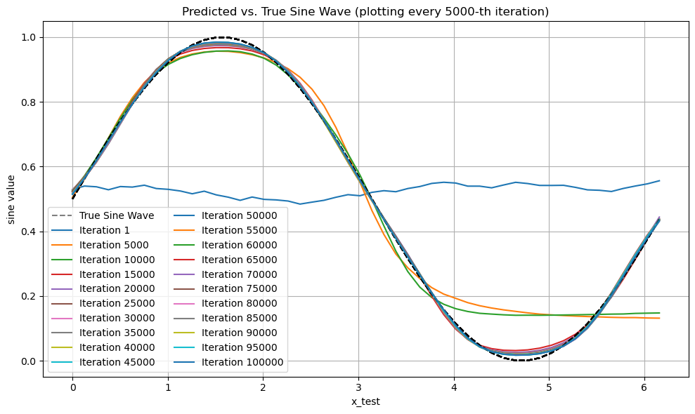
Plot the Neural Network Predictions vs True Sine Wave

iteration_step = 5000 # Plot every iteration_step iteration
iteration_list = mse_by_iter.index.to_list()
iterations_to_plot = [1] + list(range(iteration_step, iteration_list[-1]+1, iteration_step))

plt.figure(figsize=(10, 6))
for iteration in iterations_to_plot:
    group_df = grouped.get_group(iteration)

    plt.plot(group_df["x_test"], group_df["y_test"], 'k--', alpha=0.5,
                 label="True Sine Wave")
    plt.plot(group_df["x_test"], group_df["y_pred"], label=f"Iteration {iteration}")

plt.xlabel("x_test")
plt.ylabel("sine value")
plt.title(f"Predicted vs. True Sine Wave (plotting every {iteration_step}-th iteration)")
# Avoid repeated legend entries for the 'True Sine' if multiple lines are drawn
handles, labels = plt.gca().get_legend_handles_labels()
# Filter out duplicates by building an ordered dictionary
from collections import OrderedDict
by_label = OrderedDict(zip(labels, handles))
plt.legend(by_label.values(), by_label.keys(), loc="lower left", ncol=2)

plt.grid(True)
plt.tight_layout()
plt.show()

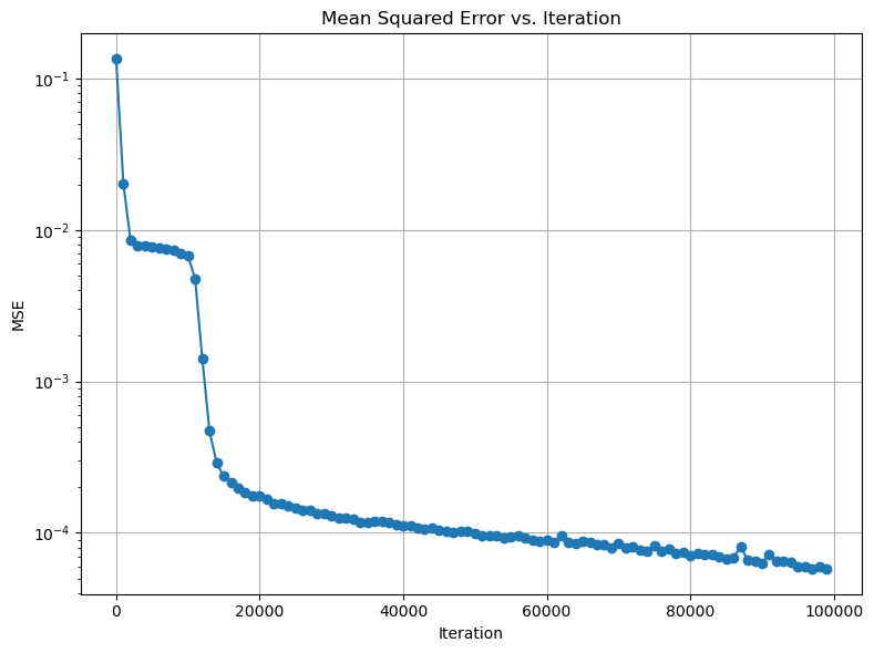
Plot the Mean Squared Error vs Iteration

plt.figure(figsize=(8, 6))
plt.plot(mse_by_iter.index[::1000], mse_by_iter.values[::1000], marker='o')
plt.title("Mean Squared Error vs. Iteration")
plt.xlabel("Iteration")
plt.ylabel("MSE")
plt.grid(True)
plt.tight_layout()
plt.yscale("log")
plt.show()

Conclusion

We have successfully trained a neural network to approximate the sine function. The neural network was implemented in Fortran using the Neural Fortran library. The data was written to a CSV file using the CSV Fortran library. The neural network predictions and mean squared error were plotted using Python.

As can be seen from the plot, the neural network was able to approximate the sine function quite well. The mean squared error decreased over time as the neural network was trained. This example demonstrates how neural networks can be used to approximate complex functions such as the sine function.

As the iteration number reached 100,000, the neural network predictions closely matched the true sine wave function. The mean squared error decreased over time as the neural network was trained. This example demonstrates how neural networks can be used to approximate complex functions such as the sine function.

A great improvement on this code would be to implement the training loop using OpenMP. This would allow the training loop to be parallelized and run on multiple cores.